Download
1 / 27
270 likes | 349 Views
Regional Climate Simulations of summer precipitation over the United States and Mexico. Kingtse Mo, Jae Schemm, Wayne Higgins, and H. K. Kim. Goals. Model resolution: Regional dependent What is the horizontal/vertical resolution needed to have skillful forecasts?

E N D
Regional Climate Simulations of summer precipitation over the United States and Mexico Kingtse Mo, Jae Schemm, Wayne Higgins, and H. K. Kim
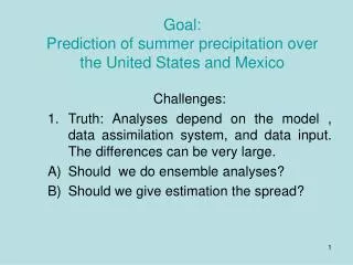
Goals • Model resolution: Regional dependent • What is the horizontal/vertical resolution needed to have skillful forecasts? • b) Importance of the initial conditions • Is this just soil moisture ? What is the best way to make summer precipitation forecasts ?
Experiments • Model : T126L28 GFS simulations with observed SSTs • Two sets of experiments: • 2 AMIP runs from 1981-2000: SAS and RAS convection schemes; • Ensemble seasonal simulations from June 29/30 each year and run through 30 September from 1990-2001. 5- member ensemble • Model: T62L64 GFS simulations • Two sets of experiments • 1). AMIP runs from 1950-2001: SAS convection scheme; • 2). Ensemble seasonal simulations from June 29/30 each year and run through 30 September from 1990-2001. 5- member ensemble The AMIP run does not have information on initial conditions , but ensemble simulations do
GFS Resolution and Precipitation in the Core Monsoon Region Precipitation (mm day-1) (1981-2000) AMIP obs T126 T62 month Kim et al(2004)
200 hPa streamline for CDAS, T62 and T126 ensemble for 1988 and 1993 as examples. • The T62 does not recognize the Gulf of California • no moisture surges, • too dry over the SW, • circulation change leads to unrealistic monsoon circulation • negative feedback to monsoon rainfall
T62 obs T126 AMIP (90-100W,36-48N)
P observed, SIMU and AMIP • AMIP126 is too dry, AMIP62 is wetter, but has no skill. • Both SIMU126 and SIMU62 give reasonable amounts of P. • Corr (obs, SIMU62)=0.57 • Corr(obs,SIMU126)=0.58 • Near the 5% statistical significant level.
P (JAS) & T2m from observations, AMIP126 and SIMU126 In comparison with observations: The AMIP is too hot (2 C higher) and too dry (2 mm/day less ) over the Great Plains ; The SIMU ensemble means are closer to the observations
P (JAS) and T2m from observations, AMIP62 and SIMU62 The T62L64 model is less drier and cooler over southern Texas, but it is too dry over the Southwest. The differences between SIMU126 and SIMU62 are small comparing to the differences between AMIP126 and AMIP62
Ensemble SIMU - AMIP 1990-2000 for T126L28 1. Over the central US: In comparison with AMIP, the ensemble SIMU has High soil moisture from the top level more E less sensible heat cooler T2m 2. More E more P, (DQ is small ) More E more P 3. Relationship is also true for the T62L64 model, but the E (and P) over the central US is 1 mm/day less.
Does the AMIP126 dry out when the model runs forward? • The comparison of SM (JAS) averaged from 1981-2000 between the regional reanalysis and AMIP shows • After winter, the May SM shows only 5% difference between the RR and the AMIP; • This rate is nearly the same as summer progresses, the AMIP126 does not dry out when summer progresses.
The AMIP126 produces less E when the summer progresses The AMIP126 does not sustain E: It is 0.5-1 mm/day less in May, but in August, the E difference increases to almost 2 mm/day or higher. The model does not lose SM that much, but it loses E badly
Soil10cm and E for 1950-2001 for AMIP62 Soil10cm from AMIP62 and AMIP126 are similar, but AMIP62 has 1mm/day more E over the central US in comparison with T126 Over the Southwest, no P no E
Mean soil10cm and E over the Northern Plains (90-100W,36-48W) E Soil10cm • Soil 10CM • AMIPs lacks variability in Soil 10cm • Simulations have more Soil10cm, but the difference is only 0.03 • E: • Large similarity between SIMU126 and SIMU62; • T62 gives higher level of E for the same Soil10cm • AMIPs lack of variability in E RR AMIP126 SIMU126 AMIP62 SIMU62 Black (Jul) Red (August) Green (sep)
For AMIP (Blue) and the RR (Green), each summer month (June-September) is one dot, For SIMU (Red), each summer month (July-September) each member in the ensemble is one red cross E is not only a function of soil moisture, it also depends on other energy terms and circulations The mean SM is around 0.21 so AMIP: E=1.75 +22.6*(SM-0.21) RR: E=3.28+27.5*(SM-0.21) SIMU: E= 1.73+25.1*(SM-0,21)
Importance of initial conditions on P fcsts over central US • Vertical resolution improves the E/SM relationship. • Accurate initial conditions are important not just because realistic soil moisture. They give realistic circulation anomalies and energy balance terms to take advantage of soil conditions, • AMIP is not upper limit of forecast skill. • Improve of surface data set like using satellite derived weekly vegetation fraction may help
Conclusions • Seasonal forecast is not just a boundary condition problem. The initial conditions are also important; • Initial SM gives interannual variability and increase fcst skill
Can we improve simulations by downscaling? Experiments: Season forecasts for 4 cases based on • A) T126L28 GFS Model (approx 80 km) • B) T62L28 GFS model (approx 200 km) • C) T62 with RSM80 downscaling (80km) • Impact of downscaling: T126 vs T62/RSM80 CASES shown :1988JJA, 1993 JAS, 1999JAS and 2000JAS with observed SSTs
Seasonal mean P from unified P data Observed Precipitation 1993-1988 1999-2000 1988 : Drought; 1993: Floods Difference: classic 3 cell pattern 1999: wet SW monsoon; 2000: dry SW T62 ensemble mean ( 8 members) 1993-1988 1999-2000 T62 model It captures P over the Central US, but it is too coarse to simulate monsoon rainfall over the SW.
Season mean P from T126 ensemble simulations Ensemble P simulations from the T126 GFS 1999-2000 1993-1988 The T126 model captures the 1988 drought and the 1993 floods and gives more realistic monsoon rainfall over the SW. RSM/T62 enesmble RSM80/T62 simulations Overall P simulation improves by downscaling, but RSM can not correct errors from T62 and improve P over the NAME region.
Conclusions • If the global forecast is good, the RSM is better • If the global forecast is not realistic, then the RSM downscaling will not correct the global model errors and improve fcsts.
July 1999 SIB RSM simulations SIB USGS The Southwest & Texas are way too dry USGS has more E over AZNM and stronger LLJ from G. of Calif
Conclusions • Over the Southwest,the impact of E to P is not large. E and P can not sustain locally. • It depends on the large scale circulation. • The horizontal resolution has to be ;large enough to resolve the Gulf of California, the LLJ and moisture transport