Download
1 / 57
570 likes | 572 Views
Learn about sorting algorithms and their importance in organizing data. Explore examples of sorting and understand algorithms such as Selection Sort, Insertion Sort, and Bubble Sort. Discover the time complexities and analysis of these algorithms.

E N D
Sorting • Sorting is a process that organizes a collection of data into either ascending or descending order. • Formally • Input: A sequence of n numbers <a1,a2,…,an> • Output: A reordering <a’1,a’2,…,a’n> of the sequence such that a’1 ≤ a’2 ≤ … ≤ a’n • Given the input <6, 3, 1, 7>, the algorithm should produce <1, 3, 6, 7> • Called an instance of the problem
Sorting • Sorting is a process that organizes a collection of data into either ascending or descending order. • We encounter sorting almost everywhere: • Sorting prices from lowest to highest • Sorting flights from earliest to latest • Sorting grades from highest to lowest • Sorting songs based on artist, album, playlist, etc.
Sorting Algorithms • There are many sorting algorithms (as of 27.10.2014 there are 44 Wikipedia entries) • In this class we will learn: • Selection Sort • Insertion Sort • Bubble Sort • Merge Sort • Quick Sort • Bogo sort and Sleep sort are some bad/slow algorithms • These are among the most fundamental sorting algorithms
Sorting Algorithms • As we learnt in the Analysis lecture (time complexity), a stupid approach uses up computing power faster than you might think. • Sorting a million numbers: • Interactive graphics: Algorithms must terminate in 1/30 of a sec.
Sorting Algorithms • As we learnt in the Analysis lecture (time complexity), a stupid approach uses up computing power faster than you might think. • Sorting a million numbers: • https://youtu.be/kPRA0W1kECg
Selection Sort • Partition the input list into a sorted and unsorted part (initially sorted part is empty) • Select the smallest element and put it to the end of the sorted part • Increase the size of the sorted part by one • Repeat this n-1 times to sort a list of n elements
Sorted Unsorted Original List After pass 1 After pass 2 After pass 3 After pass 4 After pass 5
Selection Sort (cont.) template <class Item> void selectionSort(Item a[], int n) { for (int i = 0; i < n-1; i++) { int min = i; for (int j = i+1; j < n; j++) if (a[j] < a[min]) min = j; swap(a[i], a[min]); } } template < class Object> void swap( Object &lhs, Object &rhs ) { Object tmp = lhs; lhs = rhs; rhs = tmp; }
Selection Sort -- Analysis • What is the complexity of selection sort? • Does it have different best, average, and worst case complexities?
Selection Sort – Analysis (cont.) • Selection sort is O(n2) for all three cases (prove this) • Therefore it is not very efficient
Insertion Sort • Insertion sort is a simple sorting algorithm that is appropriate for small inputs. • Most common sorting technique used by card players. • Again, the list is divided into two parts: sorted and unsorted. • In each pass, the first element of the unsorted part is picked up, transferred to the sorted sublist, and inserted at the appropriate place. • A list of n elements will take at most n-1 passes to sort the data.
Sorted Unsorted Original List After pass 1 After pass 2 After pass 3 After pass 4 After pass 5
Insertion Sort Algorithm template <class Item> void insertionSort(Item a[], int n) { for (int i = 1; i < n; i++) { Item tmp = a[i]; // the element to be inserted int j; for (j=i; j>0 && tmp < a[j-1]; j--) a[j] = a[j-1]; // shift elements a[j] = tmp; // insert } }
Insertion Sort – Analysis • Running time depends on not only the size of the array but also the contents of the array. • Best-case: O(n) • Array is already sorted in ascending order. • Worst-case: O(n2) • Array is in reverse order: • Average-case: O(n2) • We have to look at all possible initial data organizations.
Analysis of insertion sort • Which running time will be used to characterize this algorithm? • Best, worst or average? • Worst: • Longest running time (this is the upper limit for the algorithm) • It is guaranteed that the algorithm will not be worse than this. • Sometimes we are interested in average case. But there are some problems with the average case. • It is difficult to figure out the average case. i.e. what is average input? • Are we going to assume all possible inputs are equally likely? • In fact for most algorithms average case is same as the worst case.
Bubble Sort • Repeatedly swap adjacent elements that are out of order. • https://youtu.be/vxENKlcs2Tw • Sort pairs of elements far apart from each other, then progressively reduce the gap between elements to be compared. Starting with far apart elements, it can move some out-of-place elements into position faster than a simple nearest neighbor exchange. This generalization is called Shell Sort.
Bubble Sort Algorithm template <class Item> void bubleSort(Item a[], int n) { bool sorted = false; int last = n-1; for (int i = 0; (i < last) && !sorted; i++){ sorted = true; for (int j=last; j > i; j--) if (a[j-1] > a[j]{ swap(a[j],a[j-1]); sorted = false; // signal exchange } } }
Bubble Sort – Analysis • Best-case: O(n) • Array is already sorted in ascending order. • Worst-case: O(n2) • Array is in reverse order: • Average-case: O(n2) • We have to look at all possible initial data organizations. • In fact, any sorting algorithm which sorts elements by swapping adjacent elements can be proved to have an O(n2) average case complexity
Theorem • Any sorting algorithm which sorts elements by swapping adjacent elements can be proved to have an O(n2) average case complexity • To understand this, consider the following array: • [3, 2, 1] • Here, we have three inversions: (3, 2), (3, 1), (2, 1) • An inversion is defined as a pair (a, b) where a > b and index(a) < index(b) • Note that a single swap of adjacent elements can only remove one inversion. Thus, for the above example we need 3 swaps to make the array sorted
Theorem • Generalizing this, for an array of n elements, there can be C(n,2) total pairs (where C represents combination) • C(n,2) = n(n-1) / 2 • We can assume that, on average, half of these pairs are inversions. • Average number of inversions = n(n-1) / 4 • As each swap of adjacent elements can remove a single inversion, we need n(n-1) / 4 swaps to remove all inversions (that is to make the array sorted) • The complexity of n(n-1) / 4 swaps is equal to O(n2) • This is the lower bound on the average case complexity of sorting algorithms that sort by swapping adjacent elements
Recursive Insertion Sort • To sort A[1..n], we recursively sort A[1..n-1] and then insert A[n] into the sorted array A[1..n-1] • A good practice of recursion • Code?
Recursive Insertion Sort • To sort A[1..n], we recursively sort A[1..n-1] and then insert A[n] into the sorted array A[1..n-1] • insertionSortRec(A, n) • { • if (n>1) • insertionSortRec(A, n-1) • insertKeyIntoSubarray(A[n], A[1..n-1]) //trivial; can //be done in //O(n) • }
Recursive Insertion Sort • To sort A[1..n], we recursively sort A[1..n-1] and then insert A[n] into the sorted array A[1..n-1] • A = 5 2 4 6 1 3 insertKeyIntoSubarray 1 2 4 5 6 3 2 4 5 6 1 2 4 5 6 2 5 4 5 2
Recursive Insertion Sort • To sort A[1..n], we recursively sort A[1..n-1] and then insert A[n] into the sorted array A[1..n-1] • T(n) = T(n-1) + O(n) is the time complexity of this sorting
Recursive Insertion Sort • To sort A[1..n], we recursively sort A[1..n-1] and then insert A[n] into the sorted array A[1..n-1] • T(n) = T(n-1) + O(n) • Reduce the problem size to n-1 w/ O(n) extra work • Seems to be doing O(n) work n-1 times; so O(n2) guess? • T(n) ≤ cn2 //assume holds • T(n) ≤ c(n-1)2 + dn • = cn2 -2cn + c + dn • = cn2 –c(2n -1) + dn • ≤ cn2 //because large values of c dominates d
Recurrences • How about the complexity of T(n) = T(n/2) + O(1) • Reduce the problem size to half w/ O(1) extra work • Seems to be doing O(1) work logn times; so O(logn) guess? • T(n) ≤ clogn//assume holds • T(n) ≤ c(log(n/2))+ d • = clogn– clog2 + d • = clogn– e //c can always selected to be > constant d • ≤ clogn
Recurrences • How about the complexity of T(n) = 2T(n/2) + O(n) • Reduce the problem to 2 half-sized problems w/ n extra work • Seems to be doing O(n) work logn times; so O(nlogn) guess? • T(n) ≤ cnlogn//assume holds • T(n) ≤ 2c(n/2 log(n/2))+ dn • = cnlogn– cnlog2 + dn • = cnlogn– n(c’ + d) //c’ = clog2 • ≤ cnlogn
Recurrences • How about the complexity of T(n) = T(n-1) + T(n-2) • Reduce? the problem to a twice bigger one w/ no extra work • T(n-1) + T(n-2) > 2T(n-2) n replaced by 2n-4 (doubled) • Or, n-size problem replaced with 2n-3 size problem (doubled) • Seems to be doubling the problem size; so O(2n) is good guess
Fast Algorithm • Describe an algorithm that, given a set S of n integers and another integer x, determines whether or not there exists 2 elements in S whose sum is exactly x • O(n2) //brute force
Fast Algorithm • Describe an algorithm that, given a set S of n integers and another integer x, determines whether or not there exists 2 elements in S whose sum is exactly x • O(nlogn) //sort followed by binary search
Mergesort • Mergesort algorithm is one of two important divide-and-conquer sorting algorithms (the other one is quicksort). • It is a recursive algorithm. • Divides the list into halves, • Sort each halve separately (recursively), and • Then merge the sorted halves into one sorted array. • https://youtu.be/es2T6KY45cA
Mergesort - Example divide divide divide divide divide divide divide merge merge merge merge merge merge merge
Merge const int MAX_SIZE = maximum-number-of-items-in-array; void merge(DataType theArray[], int first, int mid, int last) { DataType tempArray[MAX_SIZE]; // temporary array int first1 = first; // beginning of first subarray int last1 = mid; // end of first subarray int first2 = mid + 1; // beginning of second subarray int last2 = last; // end of second subarray int index = first1; // next available location in tempArray for ( ; (first1 <= last1) && (first2 <= last2); ++index) if (theArray[first1] < theArray[first2]) tempArray[index] = theArray[first1++]; else tempArray[index] = theArray[first2++];
Merge (cont.) // finish off the first subarray, if necessary for (; first1 <= last1; ++first1, ++index) tempArray[index] = theArray[first1]; // finish off the second subarray, if necessary for (; first2 <= last2; ++first2, ++index) tempArray[index] = theArray[first2]; // copy the result back into the original array for (index = first; index <= last; ++index) theArray[index] = tempArray[index]; }
Mergesort void mergesort(DataType theArray[], int first, int last) { if (first < last) { // more than one item int mid = (first + last)/2; // index of midpoint mergesort(theArray, first, mid); mergesort(theArray, mid+1, last); // merge the two halves merge(theArray, first, mid, last); } } // end mergesort
Analysis of Mergesort • What is the complexity of the merge operation for merging two lists of size n/2? • It is O(n) as we need to copy all elements • Then the complexity of mergesort can be defined using the following recurrence relation: T(n) = 2T(n/2) + n • Solving this relation gives us O(nlogn) complexity //Slide 30 • The complexity is the same for the best, worst, and average cases • The disadvantage of mergesort is that we need to use an extra array for the merge operation (not memory efficient)
Analysis of Mergesort • Solving T(n) = 2T(n/2) + n gives us O(nlogn) complexity
Merging Step (Linear time) • Extra array for merge operation
Demo • On array = {5, 2, 4, 7, 1, 3, 2, 6}
Quicksort • Like mergesort, quicksort is also based on the divide-and-conquer paradigm. • But it uses this technique in a somewhat opposite manner, as all the hard work is done before the recursive calls. • It works as follows: • First selects a pivot element, • Then it partitions an array into two parts (elements smaller than and greater than or equal to the pivot) • Then, it sorts the parts independently (recursively), • Finally, it combines the sorted subsequences by a simple concatenation. • https://youtu.be/vxENKlcs2Tw
Partition • Partitioning places the pivot in its correct place position within the array. • Arranging the array elements around the pivot p generates two smaller sorting problems. • sort the left section of the array, and sort the right section of the array. • when these two smaller sorting problems are solved recursively, our bigger sorting problem is solved.
Pivot Selection • Which array item should be selected as pivot? • Somehow we have to select a pivot, and we hope that we will get a good partitioning. • If the items in the array arranged randomly, we choose a pivot randomly. • We can choose the first or last element as the pivot (it may not give a good partitioning). • We can choose the middle element as the pivot • We can use a combination of the above to select the pivot (in each recursive call a different technique can be used)
Partitioning Initial state of the array
Partitioning Moving theArray[firstUnknown] into S1 by swapping it with theArray[lastS1+1] and by incrementing both lastS1 and firstUnknown.
Partitioning Moving theArray[firstUnknown] into S2 by incrementing firstUnknown.