Download
1 / 62
640 likes | 813 Views
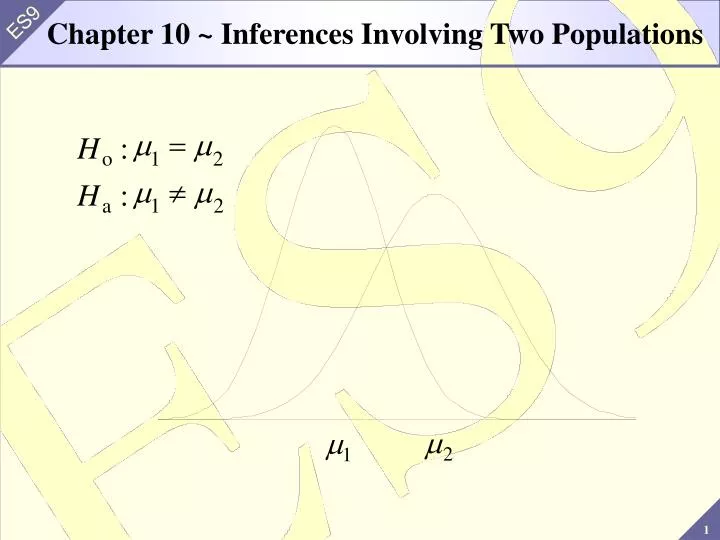
Chapter 10 ~ Inferences Involving Two Populations. m. =. m. H. :. o. 1. 2. m. ¹. m. H. :. a. 1. 2. Chapter Goals. Independent versus dependent samples. Compare two populations using: the mean of the paired differences, the difference between two means,

E N D
Chapter 10 ~ Inferences Involving Two Populations m = m H : o 1 2 m ¹ m H : a 1 2
Chapter Goals • Independent versus dependent samples • Compare two populations using: • the mean of the paired differences, • the difference between two means, • the difference between two proportions, and • the ratio of two variances
10.1 ~ Independent and Dependent Samples • Two basic kinds of samples: independent and dependent • The dependence or independence of two samples is determined by sources used for the data
Important Definitions Source: Can be a person, an object, or anything that yields a piece of data Dependent Sampling: The same set of sources or related sets are used to obtain the data representing both populations Independent Sampling: Two unrelated sets or sources are used, one set from each population
Example • Example: An experiment is designed to study the effect of classical music on mathematical ability. Thirty-five students are selected at random and given a basic mathematics skills test. The following day the same 35 students first listen to 45 minutes of classical music, and then take a similar mathematics skills test. This sampling plan illustrates dependent sampling. The sources used for both samples (without classical music and with classical music) are the same. Note: Typically, when both a pretest and a posttest are used, the same subjects are used in the study. Thus, this kind of sampling plan usually leads to dependent samples.
Example • Example: A university would like to compare the math SAT scores of male and female first-year students. Fifty males and 40 females are selected at random and their math SAT scores are recorded. This sampling plan illustrates independent sampling. The sources (students) used for each sample (male and female) were selected separately.
Example • Example: The number of items produced by two different assembly lines is to be compared. Twenty five days are randomly selected for assembly line 1 and the number of items produced on each day is recorded. Forty randomly selected days for assembly line 2 are selected and the number of items produced on each day is recorded. This sampling plan illustrates independent sampling. The sources (assembly lines) used for each sample (line 1 and 2) were selected separately.
10.2 ~ Inferences Concerning theMean Difference Using Two Dependent Samples • When dependent samples are involved, the datais paired data • Paired data results from: • Before and after studies, • A common source, and/or • Matched pairs
Paired Difference Paired difference: 1. Removes the effect of otherwise uncontrolled factors 2. The difference between the two population means, when dependent samples are used, is equivalent to the mean of the paired differences 3. An inference about the mean of the paired differences is an inference about the difference of two means 4. The mean of the sample paired differences is used as a point estimate for these inferences
Sampling Distribution of d 1. When paired observations are randomly selected from normal populations, the paired difference, d = x1-x2, will be approximately normally distributed about a mean md with a standard deviation sd 2. Use a t-test for one mean: make an inference about an unknown mean (md) where d has an approximately normal distribution with an unknown standard deviation (sd) 3. Inferences are based on a sample of n dependent pairs of data and the t distribution with n - 1 degrees of freedom The assumption for inferences about the mean of paired differences (md): The paired data are randomly selected from normally distributed populations
Confidence Interval s s - + = - d d d to d , where df n 1 t(df,a/2) t(df,a/2) n n where is the mean of the sample differences: and sd is the standard deviation of the sample differences: Confidence Interval: The 1 -a confidence interval for estimating the mean difference md is found using the formula:
Example • Example: Salt-free diets are often prescribed for people with high blood pressure. The following data was obtained from an experiment designed to estimate the reduction in diastolic blood pressure as a result of following a salt- free diet for two weeks. Assume diastolic readings to be normally distributed. Find a 99% confidence interval for the mean reduction
Solution 3. Sample evidence Sample information: 1. Population Parameter of InterestThe mean reduction (difference) in diastolic blood pressure 2. The Confidence Interval Criteria a. Assumptions: Both sample populations are assumed normal b. Test statistic: t with df = 8 - 1 = 7 c. Confidence level: 1 -a = 0.99
Solution Continued 4. The Confidence Interval a. Confidence coefficients: Two-tailed situation, a/2 = 0.005t(df, a/2) = t(7, 0.005) = 3.50 b. Maximum error: c. Confidence limits: s æ 2 . 39 ö = = = = d E 3 . 50 ( 3 . 50 )( 0 . 845 ) 2 . 957 t(df,a/2) ç ÷ è ø n 8 5. The Results -1.957 to 3.957 is the 99% confidence interval for md
Hypothesis Testing • Example: The corrosive effects of various chemicals on normal and specially treated pipes were tested by using a dependent sampling plan. The data collected is summarized by where d is the amount of corrosion on the treated pipe subtracted from the amount of corrosion on the normal pipe Hypothesis Testing: When testing a null hypothesis about the mean difference, the test statistic is: where t* has a t distribution with df = n- 1
Example Continued • Example: (Continued) Does this sample provide sufficient evidence to conclude the specially treated pipes are more resistant to corrosion? Use a = 0.05 a. Solve using the p-value approach b. Solve using the classical approach Solution: 1. The Set-up a. Population parameter of concern: The mean difference in corrosion, normal pipe - treated pipe b. The null and alternative hypothesis: Ho: md = 0 (£) (did not lower corrosion)Ha: md > 0 (did lower corrosion)
Solution Continued 3. The Sample Evidence a. Sample information: b. Calculate the value of the test statistic: 2. The Hypothesis Test Criteria a. Assumptions: Assume corrosion measures are approximately normal b. Test statistic: c. Level of significance: a = 0.05
Solution Continued 4. The Probability Distribution (p-Value Approach) a. The p-value: b. The p-value is smaller than the level of significance, a ~ or ~ = > = < P P ( t * 4 . 896 , with df 16 ) 0 . 0001 4. The Probability Distribution (Classical Approach) a. Critical value: t(16,0.05) = 1.75 b. t* is in the critical region 5. The Results a. Decision: Reject Ho b. Conclusion: At the 0.05 level of significance, there is evidence to suggest the treated pipes do not corrode as much as the normal pipes when subjected to chemicals
10.3 ~ Inferences Concerning the DifferenceBetween Means Using Two Independent Samples • Inferences based on • When comparing the means of two populations, consider the difference between their means:m1 - m2
Distribution of Distribution of : If independent samples of sizes n1 and n2 are drawn randomly from large populations with means m1 and m2 and variances and , respectively, the sampling distribution of , the difference between the sample means, has x1 - x2 2 s 2 s 1 2 - x x 1 2 1. a mean, m = m - m - 1 2 x x 1 2 æ ö æ ö 2 2 s s 2. a standard error, ç ÷ ç ÷ s = + 1 2 ç ÷ ç ÷ - x x n n è ø è ø 1 2 1 2 If both populations have normal distributions, then the sampling distribution of will also be normally distributed - x x 1 2 x1 - x2
Notes 1. Preceding statement is true for all sample sizes if the populations are normal and the population variances are known 2. Population variances are usually unknown quantities 3. Estimate the standard error by using the sample variances The assumptions for inferences about the difference between two Means m1 - m2 : The samples are randomly selected from normally distributed populations, and the samples are selected in an independent manner
Notes (Continued) No assumptions are made about the population variances The t distribution will be used as the test statistic: Case 1: t distribution, df calculated Used when a computer and statistical software computes the number of degrees of freedom. df is a function of both sample sizes and their relative sizes, and both sample variances and their relative sizes. Case 2: t distribution, df approximated Used when completing the inference without the aid of statistical software that computes df. Use the t distribution with the smaller of df1 = n1- 1 or df2 = n2- 1 degrees of freedom. This will give conservative results. The true level of confidence for an interval will be slightly higher. The true p-value and true level of significance will be slightly less than reported.
Note & Confidence Intervals æ ö æ ö 2 2 s s ç ÷ ç ÷ + 1 2 ç ÷ ç ÷ - ( ) n n t(df,a/2) è ø è ø - x x x x 1 2 1 1 2 2 æ ö æ ö 2 2 s s ç ÷ ç ÷ + 1 2 ç ÷ ç ÷ + to ( ) n n t(df,a/2) è ø è ø - 1 2 Note: When the difference between A and B is being discussed, it is customary to express the difference as larger subtract smaller so that the resulting difference is positive, A-B > 0 Confidence Intervals: The following formula is used for calculating the endpoints of the 1 -a confidence interval: where df is the smaller of df1 or df2 if df is not calculated
Example • Example: A recent study reported the longest average workweeks for non-supervisory employees in private industry to be chef and construction Find a 95% confidence interval for the difference in mean length of workweek between chef and construction. Assume normality for the sampled populations and that the samples were selected randomly. Solution: 1. Parameter of interestThe difference between the mean hours/week for chefs and the mean hours/week for construction workers, m1 - m2
Solution Continued 3. The Sample Evidence Sample information given in the table Point estimate for m1 - m2: = - = 48 . 2 44 . 1 4 . 1 - x x 1 2 2. The Confidence Interval Criteria a. Assumptions: Both populations are assumed normal and the samples were random and independently selected b. Test statistic: t with df = 11; the smaller of n1- 1 = 18 - 1 = 17 or n2- 1 = 12 - 1 = 11 c. Confidence level: 1 -a = 0.95 4. The Confidence Interval a. Confidence coefficients: t(df, a/2) = t(11, 0.025) = 2.20 (Table 6, Appendix B)
Solution Continued æ ö æ ö 2 2 s s ç ÷ ç ÷ + 1 2 ç ÷ ç ÷ n n è ø è ø 1 2 c. Confidence limits: ± = ± ( ) E 4 . 1 3 . 77 - x x 1 2 - + 4 . 1 3 . 77 to 4 . 1 3 . 77 0. 33 to 7 . 87 b. Maximum error: = t(df,a/2) E æ ö æ ö 2 2 6 . 7 2 . 3 ç ÷ ç ÷ = + = = ( 2 . 20 ) ( 2 . 20 )( 1 . 7131 ) 3 . 77 ç ÷ ç ÷ 18 12 è ø è ø 5. The Results 0.33 to 7.87 is a 95% confidence interval for the difference in mean hours/week for chefs and construction workers
Notes 1. Using a calculated df, the confidence interval is 0.55 to 7.65 2. This confidence interval is narrower than the approximate interval computed on the previous slide. This illustrates the conservative (wider) nature of the confidence interval when approximating the degrees of freedom.
Hypothesis Tests - x x 1 2 • To test a null hypothesis about the difference between two population means, use the test statistic m - m - ( ) ( ) 1 2 = t * æ ö æ ö 2 2 s s ç ÷ ç ÷ + 1 2 ç ÷ ç ÷ n n è ø è ø 1 2 where df is the smaller of df1 or df2 when computing t* without the aid of statistical software Note: The hypothesized difference between the two population means m1-m2 can be any specified value. The most common value is zero.
Example • Example: A recent study compared a new drug to ease post- operative pain with the leading brand. Independent random samples were obtained and the number of hours of pain relief for each patient were recorded. The summary statistics are given in the table below: • Is there any evidence to suggest the new drug provides longer relief from post-operative pain? Use a = 0.05 a. Solve using the p-value approach b. Solve using the classical approach
Solution 1. The Set-up a. Parameter of concern: The difference between the mean time of pain relief for the new drug and that for the leading brand b. The null and alternative hypotheses:Ho: m1-m2 = 0 (new drug relieves pain no longer)Ha: m1-m2 > 0 (new drug works longer to relieve pain) 2. The Hypothesis Test Criteria a. Assumptions: Both populations are assumed to be approximately normal. The samples were random and independently selected. b. Test statistic: t*, df = 9 df = smaller of n1- 1 = 10 - 1 = 9 or n2- 1 = 17 - 1 = 16 c. Level of significance: a = 0.05
Solution Continued - x x 1 2 3. The Sample Evidence a. Sample information: Given in the table b. Test statistic: m m - - - - ( ) ( ) ( 4 . 350 3 . 929 ) ( 0 . 00 ) 1 2 = = t * æ ö æ ö æ ö æ ö 2 2 2 2 s s 0 . 542 0 . 169 ç ÷ ç ÷ ç ÷ ç ÷ + + 1 2 ç ÷ ç ÷ ç ÷ ç ÷ n n 10 17 è ø è ø è ø è ø 1 2 0 . 421 0 . 421 = = = 2 . 39 + 0 . 0294 0 . 0017 0 . 1763
Solution Continued 4. The Probability Distribution (p-Value Approach) a. The p-value:b. The p-value is smaller than the level of significance, a = > = = P P ( t * 2 . 39 , with df 9 ) 0 . 019 ~ or ~ 4. The Probability Distribution (Classical Approach) a. Critical value: t(df, 0.05) = t(9, 0.05) = 1.83b. t* is in the critical region 5. The Results a. Decision: Reject Ho b. Conclusion: There is evidence to suggest that the new drug provides longer relief from post-operative pain at the 0.05 level of significance
Note Note: Here are the results using Minitab: Two sample T for New Drug vs Leading Brand N Mean StDev SE Mean New Drug 10 4.350 0.542 0.17 Leading 17 3.929 0.169 0.041 95% CI for mu New Drug - mu Leading: ( 0.03, 0.813) T-Test mu New Drug = mu Leading (vs >):T = 2.39 P = 0.019 DF = 10
10.4 ~ Inferences Concerning the Difference Between Proportions Using Two Independent Samples • Often interested in making statistical comparisons between two proportions, percentages, or probabilities associated with two populations
Difference Between Proportions (Continued) 1. The observed probability is where x is the number of observed successes in n trials 2. 3. p is the probability of success on an individual trial in a binomial probability experiment of n repeated independent trials Point Estimate: The difference between the observed proportions: Recall: The properties of a binomial experiment Goal: To compare two population proportions
Sampling Distribution Sampling Distribution: If independent samples of sizes n1 and n2 are drawn randomly from large populations with p1 = P1(success) and p2 = P2(success), respectively, then the sampling distribution of has these properties: 1. a mean 2. a standard error 3. an approximately normal distribution if n1 and n2 are sufficiently large
Notes & Assumptions Notes: To ensure normality: 1. The sample sizes are both larger than 20 2. The products n1p1, n1q1, n2p2, n2q2 are all larger than 5 Since p1 and p2 are unknown, these products are estimated by 3. The samples consist of less than 10% of respective populations The assumptions for inferences about the difference between two proportionsp1-p2: The n1 random observations and the n2 random observations forming the two samples are selected independently from two populations that are not changing during the sampling
Confidence Intervals Confidence Intervals: 1. A confidence interval for p1-p2 is based on the unbiased sample statistic 2. The confidence limits are found using the following formula: ¢ ¢ ¢ ¢ p q p q ¢ ¢ - z(a/2) ( p p ) - × + 1 1 2 2 1 2 n n 1 2 ¢ ¢ ¢ ¢ p q p q ¢ ¢ - z(a/2) + × + ( p p ) 1 1 2 2 to 1 2 n n 1 2
Example • Example: A consumer group compared the reliability of two similar microcomputers from two different manufacturers. The proportion requiring service within the first year after purchase was determined for samples from each of two manufacturers. Find a 98% confidence interval for p1-p2, the difference in proportions needing service
Solution 2. The Confidence Interval Criteria a. Assumptions: Sample sizes larger than 20 Products all larger than 5 should have an approximate normal distribution b. Test statistic: z* c. Confidence level: 1 -a = 0.98 1. Population Parameter of Interest: The difference between the proportion of microcomputers needing service for manufacturer 1 and the proportion of microcomputers needing service for manufacturer 2
Solution Continued 0 . 98 z(0.01) 3. The Sample Evidence Sample information: Point estimate: 4. The Confidence Interval a. Confidence coefficients:z(a/2) = z(0.01) = 2.33
Solution Continued ¢ ¢ ¢ ¢ p q p q ( 0 . 15 )( 0 . 85 ) ( 0 . 09 )( 0 . 91 ) × + = + 1 1 2 2 2 . 33 n n 200 250 1 2 c. Confidence limits b. Maximum error z(a/2) = E = + = = 2 . 33 0 . 0006375 0 . 0003276 ( 2 . 33 )( 0 . 0311 ) 0 . 0724 5. Results -0.0124 to 0.1324 is a 98% confidence interval for the difference in proportions
Hypothesis Tests Notes: 1. The null hypothesis is p1 = p2, or p1-p2 = 0 2. Nonzero differences between proportions are not discussed in this section 3. The numerator of the formula above: Hypothesis Tests:If the null hypothesis is there is no difference between proportions, the test statistic is:
Notes Continued 4. Since the null hypothesis is p1 = p2, the standard error of the point estimate is: where p = p1 = p2 and q = 1 -p 5. Use a pooled estimate for the common proportion: The test statistic becomes:
Example • Example: The proportion of defective parts from two different suppliers were compared. The following data was collected: Is there any evidence to suggest the proportion of defectives is different for the two suppliers? Use a = 0.01 a. Solve using the p-value approach b. Solve using the classical approach Solution: 1. The Set-up a. Population parameter of interest: The difference between the proportion of defectives for supplier 1 and the proportion of defectives for supplier 2
Solution Continued 2. The Hypothesis Test Criteria a. Assumptions: Populations are large (number of parts supplied) Samples are larger than 20 Products are larger than 5 Sampling distribution should be approximately normal b. Test statistic: z* c. Level of significance: a = 0.01 b. The null and alternative hypotheses: Ho: p1-p2 = 0 (proportion of defectives the same) Ha: p1-p2¹ 0 (proportion of defectives different)
Solution Continued b. Test statistic: 3. The Sample Evidence a. Sample information:
Solution Continued ~ or ~ 4. The Probability Distribution (Classical Approach) a. Critical value: z(a/2) = z(0.005) = 2.58 b. z* is not in the critical region = > = - = 1/2 P P ( z * 1 . 03 ) 0 . 5000 0 . 3485 0 . 1515 4. The Probability Distribution (p-Value Approach) a. The p-value: b. The p-value is larger than the level of significance, a = = P 2 ( 0 . 1515 ) 0 . 3030 5. The Results a. Decision: Do not reject Ho b. Conclusion: There is no evidence to suggest the proportion of defectives is different for the two suppliers at the 0.01 level of significance
10.5 ~ Inferences Concerning the Ratio of Variances Using Two Independent Samples • Compare the standard deviations of two populations • Sampling distributions dealing with sample standard deviations (or variances) are very sensitive to slight departures from the assumptions • Consider the hypothesis test for the equality of standard deviations (or variances) for two normal populations
Background 1. The hypothesis test procedure uses the ratio of variances 2. Inferences about the ratio of variances for two normally distributed populations uses the F distribution 3. The F distribution is a family of probability distributions 4. Each F distribution is identified by two numbers of degrees of freedom, one for each of the two samples involved