Download
1 / 55
560 likes | 609 Views
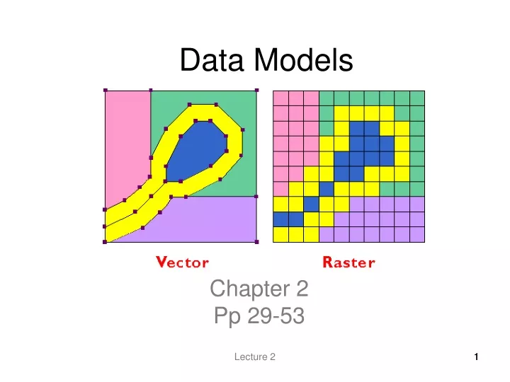
Data Models. Chapter 2 Pp 29-53. 1. Phenomena/ entities that exist in the real world. Computer Representation. Machine Code 10011101 00110110 10110100. An abstraction, relevant phenomena and properties. 2. Data Model. Objects in a spatial database.

E N D
Data Models Chapter 2 Pp 29-53 Lecture 2 1
Phenomena/entities that exist in the real world Computer Representation Machine Code 10011101 00110110 10110100 An abstraction, relevant phenomena and properties Lecture 2 2
Data Model • Objects in a spatial database. • The spatial data model provides a formal means of representing and manipulating spatially-referenced information. Lecture 2 3
Coordinates • Coordinates are used to define the location and extent of spatial objects. https://www.codeproject.com/Articles/44389/Build-a-Desktop-GIS-Application-Using-MapWinGIS Lecture 2
Attributes • Attributes describe the spatial object. • Attribute data complements the coordinate data to define the spatial object. Lecture 2
Thematic Layers • A logical separation of data according to theme. • Each layer reflects a particular use or characteristic. • Overlays. https://jessyfaas.wordpress.com/2016/07/01/gis-in-het-voortgezet-onderwijs-wat-is-gis/comment-page-1/ 6 Lecture 2
Coordinate Data • GIS often uses a Cartesian coordinate system. • Cartesian Coordinate System (x & y or x, y & z) • Usually specified as decimal numbers that increase from bottom to top. Lecture 2 7
Coordinate Data • Latitude & Longitude • Origin (intersection of the Equator and Greenwich meridian) • Spherical Coordinates • Deg., min., sec. (DMS) • Decimal degrees (DD) Lecture 2 8
Nomenclature of Geographic Coordinate System http://www.justtrails.com/nav-skills/navigation-skills-latitude-and-longitude/ Lecture 2
Conversion from Spherical to Cartesian Tissot’s Indicatrix http://www.perrygeo.com/tissot-indicatrix-examining-the-distortion-of-map-projections.html Lecture 2
Conversionfrom DMS to DD Convert: 68o 40’ 19.2” W to decimal degrees: Lecture 2 11
Conversionfrom DD to DMS 68o 48’ 57” Convert: -68.67200 to degrees, minutes, seconds: Lecture 2 12
Converting Arc to Surface Distance Where d is the ground distance, r is the radius of the sphere and the angle is specified in radians. Lecture 2
Converting Arc to Surface Distance At the equator, one degree of longitude is about 111km Lecture 2
An Ellipsoidal Earth http://qcoherent.com/newsletter/December2014/December2014_2.html Lecture 2
Great Circle A great circle is defined as any line resulting from a plane passing through the center of the globe. http://www.shsu.edu/~dl_www/bkonline/GenRef111/Reading/RefL01Maps/Lab01index.htm Lecture 2
c=a-b c a=90o-a a b=90o-b b Latitude ϕ, Longitude λ Lecture 2
Conversion from Geographic to Cartesian Coordinates This formula requires latitude and longitude to be in radians. Lecture 2
Geographic & Magnetic North http://www.ingv.it/ufficio-stampa/research-areas/the-earth/characteristics-of-the-earth-s-magnetic-field/view?set_language=en Lecture 2
Types of Attribute Data • Attribute data record the non-spatial characteristics of an entity. • Attributes have values • Observed • Measured Llbean.com Lecture 2 20
Measurement of Attributes • Physical scientists define measurement as the comparison of an object to a standard object. • They define two types of measurements • Extensive/Fundamental Properties (feet) • Derived – by combining extensive properties (feet/second) Lecture 2 21
Stevens’ Levels of Measurement • Social scientists weren’t satisfied with this classification • Stanley Stevens (1946) proposed a framework for measurement types based upon “levels of measurement”. • He defined measurement as being the assignment of classes or scores to phenomena according to a set of rules. Lecture 2 22
Stevens’ Levels of Measurement • There are four basic levels according to Stevens: • Nominal – provides descriptive information. • Ordinal – implies a rank order. • Interval – implies order and difference in magnitude. • Ratio - implies order and difference in magnitude and has an absolute 0. Lecture 2 23
Ordinal • You can do comparisons: • If A>B and B>C then the correct increasing order is C, B, A; i.e., establish order • You can establish equality between two orders. Lecture 2 Lecture 2
Interval • Operations include: • Count • Equality • Order • Addition and Subtraction Lecture 2 Lecture 2
Ratio • Operations: • Count • Equality • Order • Addition and Subtraction • Multiplication and Division • Higher order operations Lecture 2 Lecture 2
Additional Levels of Measurement • Nicholas Chrisman includes several more in his textbook "Exploring Geographic Information Systems." • I will add those here: • Absolute scales – scales bounded on both ends like probability • Cyclical measures – angular measure • Counts are misfits. They are not continuous, but otherwise behave as a ratio scale • Graded membership in categories – Fuzzy set theory; i.e., not all membership within a class must be equal. Lecture 2 Lecture 2
Spatial Data Vector Data Raster Data Non-topological Topological Higher-level Data Simple Data Dynamic Segmentation Regions TIN Common GIS Data Models Lecture 2 Lecture 2 28
Two Most Common Spatial Data Models Lecture 2 29
Triangulated Irregular Network(TIN) http://www.geosolutions.com/3d/analyse/images/interpolate_tin.gif Lecture 2
Regions https://gis1.usgs.gov/csas/gap/viewer/land_cover/Images/Regions.png Lecture 2
Dynamic Segmentation Dynamic segmentation is the process of computing the map location (shape) of events stored in an event table. Dynamic segmentation is what allows multiple sets of attributes to be associated with any portion of a linear feature. http://resources.arcgis.com/en/help/main/10.1/index.html#//003900000026000000 Lecture 2
Contour Lines over a Raster http://www4.ncsu.edu/~hmitaso/gmslab/hohen2/w2elev10.gif Lecture 2
Vector & Raster • Vector is better at representing discrete features. • Raster is better at representing continuous features • A project may contain both vector and raster layers. • Spatial operations can only be performed on one type of layer. Lecture 2 34
Vector & Raster (cont’d) • The best data model for a given layer depends upon the operations, the experience and the views of the user. • No decision is final, as one can be converted to the other. Lecture 2 35
Vector Terminology The terms polygon and area will be used interchangeably. Lecture 2 Lecture 2
Multiple Representations Lecture 2
Vector Model Lecture 2
Single Part Features 1 to 1 Relationship Lecture 2
Multipart Features Many to 1 Relationship Lecture 2
Multipart to Single-Part Problem Lecture 2
Polygon Inclusion Lecture 2
Polygon Inclusions • Areas in polygons that are part of the polygon, but different from the rest of the polygon: e.g. Islands in a lake. • Solutions: • Create separate polygons for each inclusion. • Create an attribute column for coding inclusions. Lecture 2 Lecture 2
Boundary Generalization • The incomplete representation of boundary locations. http://www.i95exitguide.com/side-trips/the-maine-coastline/ Lecture 2
Vector Topology Topology – geometric properties that to not change with shape: Adjacency, Connectivity, Containment Lecture 2
Topology Topology in the object data model is a set of rules and software tools to define spatial relationships an behaviors, such as: • Polygons must not overlap within a dataset. • Lines must not overlap themselves within a data set. Lecture 2 Lecture 2
Three Types of Vector Features Lecture 2
Advantages of Topology • Maintain correct data spatial relationship (Find errors) • Efficient data storage (quickly process large data sets) • Facilitate spatial analysis (Network analysis, Adjacent area analysis, overlay analysis Lecture 2 Lecture 2
Encoding Topological Primitives Polygon Bounding Arcs A (e,f,g,i,j) (h) (k) B (a,b,c,-i) C (-c,d,-j) D (-k) Lecture 2 Lecture 2
Arc Bounding Nodes Left Poly Right Poly a 1,2 - B b 2,3 - B c 3,5 C B d 3,4 - C … k 9,9 D A Lecture 2