Download
1 / 35
350 likes | 521 Views
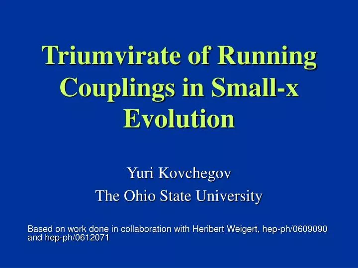
Triumvirate of Running Couplings in Small-x Evolution. Yuri Kovchegov The Ohio State University. Based on work done in collaboration with Heribert Weigert, hep-ph/0609090 and hep-ph/0612071. Preview.

E N D
Triumvirate of Running Couplings in Small-x Evolution Yuri Kovchegov The Ohio State University Based on work done in collaboration with Heribert Weigert, hep-ph/0609090 and hep-ph/0612071
Preview • Our goal here is to include running coupling corrections to BFKL/BK/JIMWLK small-x evolution equations. • The result is that the running coupling corrections come in as a “triumvirate” of couplings:
DIS in the Classical Approximation The DIS process in the rest frame of the target is shown below. It factorizes into with rapidity Y=ln(1/x)
DIS in the Classical Approximation The dipole-nucleus amplitude in the classical approximation is A.H. Mueller, ‘90 Black disk limit, Color transparency 1/QS
Quantum Evolution As energy increases the higher Fock states including gluons on top of the quark-antiquark pair become important. They generate a cascade of gluons. These extra gluons bring in powers of aS ln s, such that when aS << 1 and ln s >>1 this parameter is aS ln s ~ 1.
BFKL Equation In the conventional Feynman diagram picture the BFKL equation can be represented by a ladder graph shown here. Each rung of the ladder brings in a power of a ln s. The resulting dipole amplitude grows as a power of energy violating Froissart unitarity bound How can we fix the problem? Let’s first resum the cascade of gluons shown before.
The BFKL equation for the number of partons N reads: BFKL Equation Balitsky, Fadin, Kuraev, Lipatov ‘78 The powers of the parameter a ln swithout multiple rescatterings are resummed by the BFKL equation. Start with N particles in the proton’s wave function. As we increase the energy a new particle can be emitted by either one of the N particles. The number of newly emitted particles is proportional to N.
Resumming Gluonic Cascade In the large-NC limit of QCD the gluon corrections become color dipoles. Gluon cascade becomes a dipole cascade. A. H. Mueller, ’93-’94 We need to resum dipole cascade, with each final state dipole interacting with the target. Yu. K. ‘99
NonlinearEvolutionEquation Defining rapidity Y=ln s we can resum the dipole cascade I. Balitsky, ’96, HE effective lagrangian Yu. K., ’99, large NC QCD initial condition • Linear part is BFKL, quadratic term brings in damping
Number of parton pairs ~ Nonlinear Equation At very high energy parton recombination becomes important. Partons not only split into more partons, but also recombine. Recombination reduces the number of partons in the wave function. I. Balitsky ’96 (effective lagrangian) Yu. K. ’99 (large NC QCD)
“Phase Diagram” of High Energy QCD Saturation physics allows us to study regions of high parton density in the small coupling regime, where calculations are still under control! (or pT2) Transition to saturation region is characterized by the saturation scale
What Sets the Scale for the Running Coupling? In order to perform consistent calculations it is important to know the scale of the running coupling constant in the evolution equation. There are three possible scales – the sizes of the “parent” Dipole and “daughter” dipoles . Which one is it?
Main Principle To set the scale of the coupling constant we will first calculate the corrections to BK/JIMWLK evolution kernel to all orders. We then would complete to the QCD beta-function by replacing .
Leading Order Corrections The lowest order corrections to one step of evolution are A C B UV divergent ~ ln m UV divergent ~ ln m ?
Diagram A If we keep the transverse coordinates of the quark and the antiquark fixed, then the diagram would be finite. If we integrate over the transverse size of the quark-antiquark pair, then it would be UV divergent. ~ ln m Why do we care about this diagram at all? It does not even have the structure of the LO dipole kernel!!!
Running Coupling Corrections to All Orders Let’s insert fermion bubbles to all orders:
Virtual Diagram: Graph C Concentrating on UV divergences only we write All running coupling corrections assemble into the physical coupling .
Real Diagram: Graph B Again, concentrating on UV divergences only we write Running coupling corrections do not assemble into anything one could express in terms of the physical coupling !!!
Real Diagram: Graph A Looks like resummation without diagram A does not make sense after all. Keeping the UV divergent parts we write:
Real Diagrams: A+B Adding the two diagrams together we get Two graphs together give results depending on physical couplings only! They come in as “triumvirate”!
Extracting the UV Divergence from Graph A We can add and subtract the UV-divergent part of graph A: UV-finite + UV-divergent
Extracting the UV Divergence from Graph A In principle there appears to be no unique way to extract the UV divergence from graph A. Which coordinate should we keep fixed as we integrate over the size of the quark-antiquark pair? gluon Need to integrate over One can keep either or fixed (Balitsky, hep-ph/0609105).
Extracting the UV Divergence from Graph A gluon We decided to fix the transverse coordinate of the gluon:
Results: Transverse Momentum Space The resulting JIMWLK kernel with running coupling corrections is where q The BK kernel is obtained from the above by summing over all possible emissions of the gluon off the quark and anti-quark lines. q’
Results: Transverse Coordinate Space To Fourier-transform the kernel into transverse coordinate space one has to integrate over Landau pole(s). Since no one knows how to do this, one is left with the ambiguity/power corrections. The standard way is to use a randomly chosen (usually PV) contour in Borel plane and then estimate power corrections to it by picking the renormalon pole. This is done by Gardi, Kuokkanen, Rummukainen and Weigert in hep-ph/0609087. Renormalon corrections may be large…
Running Coupling BK Let us ignore the Landau pole for now. Then after the Fourier transform we get the BK equation with the running coupling corrections: where
A Word of Caution When we performed a UV subtraction we left out a part of the kernel. Hence the evolution equation is incomplete unless we put that UV-finite term back in. Adding the term back in removes the dependence of the procedure on the choice of the subtraction point! The numerical significance of this term is being investigated by Albacete et al.
NLO BFKL Since we know corrections to all orders, we know them at the lowest order and can find their contribution to the NLO BFKL intercept. However, in order to compare that to the results of Fadin and Lipatov and of Camici and Ciafaloni (CCFL) we need to find the NLO BFKL kernel for the same observable. Here we have been dealing with the dipole amplitude N. To compare to CCFL we need to write down an equation for the unintegrated gluon distribution.
NLO BFKL At the leading twist level we define the gluon distribution by
NLO BFKL Defining the intercept by acting with the NLO kernel on the LO eigenfunctions we get with in agreement with the results of Camici, Ciafaloni, Fadin and Lipatov! (Of course is the LO BFKL eigenvalue.)
BFKL with Running Coupling We can also write down an expression for the BFKL equation with running coupling corrections: If one rescales theunintegrated gluon distribution: then one gets in agreement with Braun (hep-ph/9408261) and Levin (hep-ph/9412345), though for a differently normalized gluon distribution.
Conclusions • We have derived the BK/JIMWLK evolution equations with the running coupling corrections. Amazingly enough they come in as a “triumvirate” of running couplings. • We have independently confirmed the results of Camici, Ciafaloni, Fadin and Lipatov for the leading-Nf NLO BFKL intercept.
Conclusions • We have derived the BFKL equation with the running coupling corrections. The answer confirms the conjecture of Braun and Levin, based on postulating bootstrap to all orders, though for the unintegrated gluon distribution with a non-traditional normalization.