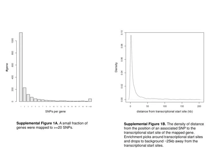
Supplemental Figure 1A. A small fraction of genes were mapped to >=20 SNPs.

1. Supplemental Figure 1A. A small fraction of genes were mapped to >=20 SNPs. Supplemental Figure 1B. The density of distance from the position of an associated SNP to the transcriptional start site of the mapped gene. Enrichment picks around transcriptional start sites and drops to background ~25kb away from the transcriptional start sites.

2. Supplemental Figure 1C. The effect for locally (red) and distantly (blue) associated SNPs.

3. Supplemental Figure 1D. Examples of genes regulated by trans hot spots. The mean relative gene expression levels were plotted against the genotypes at the three trans hot spots. C: Col allele, N: non-Col allele, where Col refers to the reference accession Columbia. Different genes were denoted by different colors.

4. Supplemental Figure 1E. Scatter plot of the first two components from principle component analysis for 57 F1 lines using SNP genotypes.

5. Supplemental Figure 1F. The effect of population structure on gene expression association. For each of the genes mapped locally (upper panels) or distantly (lower panels) at FDR < 0.2, the observed p-value across all tested SNPs were plotted against the expected p-value. Red, orange and blue lines represent the mean, one standard deviation from mean, and range, respectively, across genes. Black dashed lines represent the diagonal lines.

6. Supplemental Figure 2A. The short-range, strong LD is similar between local (solid lines) and distant (dashed lines) associations. Associations were detected at FDR < 0.4 (red), 0.3 (green), 0.2 (blue), 0.1 (cyan) and 0.05 (purple). For distant associations, the associations at the largest trans hot spot 4_14423393_C_A and the nearby 4_14423222_G_A were removed from analysis. LD block length was defined as the distance between the first two flanking SNPs, with which focal SNP r2 < 0.8. Black solid line: randomly sampled 20k SNPs. Supplemental Figure 2B. The peak of the extended LD for distant associations in Figure 1B was mostly contributed by the trans hot spot 4_14423393_C_A. The distribution of LD block length for local (solid lines) and distant (dashed lines) associations detected at FDR < 0.4 (red), 0.3 (green), 0.2 (blue), 0.1 (cyan) and 0.05 (purple). For distant associations, the associations at 4_14423393_C_A and the nearby 4_14423222_G_A were removed from analysis. LD block length was defined as the distance between the first two flanking SNPs, with which focal SNP r2 < 0.1. Black solid line: randomly sampled 20k SNPs.

7. Supplemental Figure 3A. The effect size of local eQTL were plotted along 500bp bins for upstream 25kb (-25kb to transcriptional start) and down stream 25kb (transcriptional stop to +25kb). Within gene positions were binned to 5 positional quantiles. TSS: transcriptional start site; end: transcriptional stop site. The effect size exhibits modest negative correlation with the distance to gene (p < 1.20E-19, R2=0.016 for upstream region; p < 1.96E-16, R2=0.015 for downstream region).   Supplemental Figure 3B. The clustering of associated SNPs by LD, for genes detected at FDR < 0.05 in local scan of expression level (solid bars) and for genes overlapping between ASE (q < 0.1) and expression association (dashed bars). A gene could have single eQTL (local 1) or multiple eQTL (local > 1) within local regulatory region. SNPs were clustered at LD thresholds r2 > 0.2 (black), 0.4 (red), 0.6 (green) and 0.8 (blue).

8. Leaf sample from 16 F1 lines ASE trait mapped to the local SNP Phase groups LAR sense LAR antisense Col allele non-Col allele Col allele non-Col allele Supplemental Figure 4A. An example of aseQTL association. Here suppose an ASE trait is mapped against a local SNP (red/blue stars in the upstream region of the gene). A total of 16 F1 lines are heterozygous at the transcribed SNP (yellow/green stars within the gene). For the 16 lines, 3 phase groups are determined by the allelic combination between the SNP tested for association and the transcribed SNP. ASE trait is measured as Log Allele intensity Ratio (LAR) at the transcribed SNP. The ASE trait is regressed in a linear model using the phase groups as explanatory factor, in a similar sense that gene expression trait is regressed in a linear model using genotype as explanatory factor. LAR is defined by: log ( Col-allele intensity / non-Col allele intensity ). In this example, Col allele at the regulatory SNP up-regulates the transcription of the linked allele of the target gene.

9. Supplemental Figure 4B. The density distribution of the mean gene expression level across samples, for genes detected in expression association but not in ASE association (black), and genes detected in ASE association but not in expression association (red). Detection threshold for expression association: FDR < 0.05, for ASE association: q < 0.1.

10. Supplemental Figure 4C. An example of trans-acting local eQTL. (left) The relative gene expression levels were plotted against the genotypes at the regulatory SNP 1_4357889_C_T. C: Col allele; N: non-Col allele. (right) The LARs of sense strain at transcribed SNP 1_4356154_A_G were plotted against the LARs of antisense strain. Red points: lines for which the transcribed SNP is homozygous Col allele; blue points: lines for which the transcribed SNP is homozygous non-Col allele; black points: lines for which transcribed SNP is heterozygous and the regulatory SNP is homozygous; yellow points: lines for which transcribed SNP is heterozygous and the regulatory SNP is in phase with transcribed SNP; green points: lines for which transcribed SNP is heterozygous and the regulatory SNP is out of phase with transcribed SNP.

11. Supplemental Figure 5A. Additive associations (red) have larger effect than dominant associations (blue). Supplemental Figure 5B. The percentage of genes mapped to local regulatory region only (local), a single distant region (1 distant), multiple distant regions (>1 distant), and both local and distant regions (local & distant), in GWA of genetic inheritance of gene expression. Associations were detected at FDR < 0.4 (black), 0.3 (red), 0.2 (green), 0.1 (blue) and 0.05 (cyan).

12. Supplemental Figure 5C. The d/a ratio (dominance effect / additive effect) distribution for local dominant associations (black) and distant dominant associations (red). To calculate d/a ratio, the mean expression levels for the homozygotes were ordered so that X11 > X22, where X11, X22 represent mean expression levels for homozygous genotype 1 and homozygous genotype 2, respectively. Additive effect = (X11-X22)/2, dominant effect = X12-(X11+X22)/2, where X12 represents mean expression levels for heterozygotes. (left) Associations detected at FDR < 0.2 in GWA of genetic inheritance. (right) The associations detected at FDR < 0.4 in GWA of genetic inheritance were obtained and ranked by the fold change between two homozygote genotypes.

13. Supplemental Figure 5D. Examples of genes regulated by dominant hot spots. The mean relative gene expression levels were plotted against the genotypes at four dominant hot spots. Different genes were denoted by different colors.

14. Supplemental Figure 6. Effect size for locally associated SNPs (red) and distantly associated SNPs (blue) from GWA of intron (left) and exon (right) splicing variation.