Download
1 / 33
330 likes | 415 Views
Cluster Analysis Finding Groups in Data. C. Taillie February 19, 2004. Atypical Example of Clustering. 1 2 3 4 5.

E N D
Cluster AnalysisFinding Groups in Data C. Taillie February 19, 2004
Atypical Example of Clustering 1 2 3 4 5 6 7 8 9 10 Digitized Photographs of Ten Natural Scenes Can we group them into clusters so that photos within each cluster are similar as images?
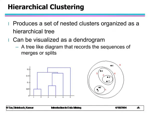
Dendrogram Dissimilarity Dendrogram for Atypical Example 1 2 3 4 5 6 7 8 9 10 Photo
Dendrogram = Many Groupings 1 2 3 4 5 6 7 8 9 10
Splitogram Dissimilarity 1 2 3 4 5 6 7 8 9 Splitting Node Splitogram:Choosing Number of Clusters 1 2 3 4 5 6 7 8 9 10 1 2 3 4 5 6 7 9 8
Atypical Example What makes this example atypical? • Splitogram levels off at a dissimilarity of about 0.6 (max=1.4)Typically, splitogram levels off to zero • Number of objects to cluster is small (only 10)Typically, number of objects is in hundreds or thousands, sometimes millions • Number of measurements per object is immense (one grey-scale value for each of several million pixels)Typically, number of measurements per object ranges from a few to a few hundred • Complicated spatial structure among the measurements and a specialized dissimilarity measure tailored to that spatial structureTypically, one uses generic dissimilarity measures likeEuclidian distance
Entomology of “Dendrogram” • Statisticians did not invent dendrograms • dendron = Tree (Greek) • gramma = Diagram (Greek) • dendrogram = Tree Diagram (specifically for classification or grouping of objects) • dendrograms have been around for aeons, especially in taxonomy
Taxonomic Dendrogram for Primates • Artistic Issues: • Is the Root at the top or bottom of the tree? (Don Knuth ……) • Ordering of the leaf nodes? Not significant, except that each cluster represents a consecutive sequence • However, ordering of leaf nodes can influence reader’s perception. Try interchanging “human” with the two “chimp” groupings!!!!
Classification vs Clustering • Classification • A priori set of labels (categories) with meaningful descriptions/interpretations so that, with sufficient effort, an “expert” could assign a given object to its true category • Landcover categories (forest, urban, desert, grassland, etc.) • Taxonomic categories (species of moths) • Set of “training” data whose objects have been expertly classified • Goal in Statistical Classification: Develop rules so that new objects can be classified without the need for an expert
Training Data with Three Categories X2 Simple Classification Rule X2 X1 X1 Classification New Object Complex Classification Rule X2 New Object X1
Classification Essential feature of Classification: Each object has a TRUE category so the performance of any classification rule can be assessed (doing so may be expensive) Test Data Inaccuracy Good Bad Best Rule Training Data Simple Complex Rules
Classification vs Clustering • Clustering • Collection of objects and a set of measurements on each object • Goal in Statistical Clustering: Divide the objects into groups so that objects in the same group are “similar” and objects in different groups are “dissimilar” Assign an identifying group label to each object. Objects with the same label belong to the same group, but a clustering algorithm attaches no other meaning or interpretation to the labels. Interpretation of the labels is up to the user. • Clustering algorithm itself does not provide a way of assigning new objects to the clusters
Three Groups X2 X1 Four Groups X2 X1 Clustering Original (ungrouped) Data X2 X1 Which of the two groupings is “correct”?
Clustering • Cluster Analysis is an Exploratory Tool • There is no notion of a TRUE cluster • Therefore, no way of evaluating the performance of a particular clustering algorithm • The only criterion is whether it yields anything useful for you
Applications of Cluster Analysis • Performance Evaluation(first few slides---unusual application) • Precursor to ClassificationAssign meaningful interpretations to cluster labels and obtain an initial training set • Reduce/Simplify a Large DatabaseDatabases in economics and commerce can be megabytes or gigabytes in size. Even something as simple as computing a mean can consume huge amounts of computer time
Database Reduction - 1 May be millions of records (rows) in database and hundreds or thousands of variables Get rid of the variables
Database Reduction - 2 Collapse every cluster to its centroid X2 X2 B A C X1 X1 Create Auxiliary Table – One row for each cluster
Ward’s Method Ward, J.H. (1963). Hierarchical groupings to optimize an objective function. J. American Statistical Society, 58, 236-244. • Within- and Between Group Sum of Squares • SSTotal = SSWithin + SSBetween • A “good” clustering should have: • Small within-group sum of squares (objects in a group should be similar) • Large between group sum of squares (objects in different groups should be dissimilar) • Bottom-up (agglomerative) hierarchical approach: • Start with each object in its own separate cluster (bottom of the dendrogram --- SSWithin = 0) • Combine clusters two at a time; at each step combine the pair of clusters that gives the smallest increase in SSWithin
Dendrogram for Ward’s Method SSTotal Within-group SS Value of SSWithinjust after the fusion 0
Other Agglomerative Hierarchical Methods • Dissimilarity measure D(a,b) between individual objectsa and b • Euclidian distance • Manhattan distance • Minkowski distance • Extend D to a measure of dissimilarity D(A,B) betweengroups of objectsA and B. This is called the linkage method: • Single linkage • Complete linkage • Average linkage • Centroid linkage • Ward’s linkage (should be called Wishart’s linkage)
Linkage Methods Link between A and B a B b A • Single linkageD(A,B) is the shortest link between A and B • Complete linkageD(A,B) is the longest link between A and B • Average linkageD(A,B) is the average of all the links between A and B • Centroid linkage • Ward’s linkage (should really be called Wishart’s linkage)Centroid linkage weighted by the cluster sizes
Ward’s Linkage Wishart showed that when groups A and B are fused, the increase in the within group sum of squares iswhere D2 is squared Euclidean distance. So it is a weighted form of centroid linkage. The weight can be rewritten as
Why is Weighting Desirable ? 10 objects 50 objects 10 objects 50 objects Which pair of group would you prefer to fuse? The pair on the left or on the right? The “sample sizes” on the right are larger so there is stronger evidence that the groups on the right are really different. We can achieve this choice by weighting centroidal distance by the average of the group sizes.
Why is Harmonic Mean Better than Arithmetic Mean ? 1 object 50 objects 99 objects 50 objects Which pair of group would you prefer to fuse? The pair on the left or on the right? The total sample sizes are the same (100) for each pair. But the “sample sizes” on the right are balanced so there is stronger evidence that the groups on the right are really different. We can achieve this choice by weighting centroidal distance by the harmonic mean of the group sizes instead of the arithmetic mean.
Classification of Clustering Methods Hierarchical Partitional Agglomerative Divisive
Agglomerative vs Divisive: Practicalities How much computer time is required with N objects? Agglomerative There are N(N-1)/2 pairs of objects, so computer time is O(N2) With N=100, O(N2) is about 10,000 With N=1,000, O(N2) is about one million With N=10,000, O(N2) is about one hundred million Divisive There are 2N-1-1 pairs of nonempty subsets, so computer time is O(2N) With N=10, O(2N) is about 1,000 With N=20, O(2N) is about one million With N=30, O(2N) is about one billion Examination of all possible subsets is hopeless unless N is very small.
Partitional Methods • The desired number of clusters, k, is specified beforehand. • Three best-known methods: • k-means (moving centroid method) • k-means (Hartigan’s method) • ISODATA (k-means with many embellishments) Available in many of the GIS and image analysis packages, e.g. ENVI
k-Means (Moving Centroids) • Specify the value of k • Specify k points (called “seeds”) in measurement space. The algorithm moves the seeds around until they are the centroids of the k desired groups. • Make a pass through the data points. Assign each data point to its closest seed. This determines a partition of the data into k groups, each labeled by its seed. However, a group’s centroid may fail to coincide with the group’s seed. • For each group, compute its centroid. Use these centroids as the seeds in the next iteration. • Keep iterating until centroids and seeds coincide (to a user- specified degree of accuracy).
k-Means (Hartigan’s Method) • Specify the value of k • Specify k nonempty starting groups. • Make a pass through the data points. • For each data point, ask if the within-group sum of squares could be reduced by moving that data point to another group. • If yes, move it; otherwise proceed to the next data point • Keep iterating until no data point can be moved. • Hartigan discovered some computationally simple rules for deciding if a data point should be moved and for finding the best group to move it to.
ISODATA Basically the same as the moving centroid version of k-means, except that the user specifies a range of acceptable values for the desired number of clusters. After each iteration of moving centroids, the current groups are examined to see if any should be split into two subgroups or fused into a larger group. These decisions are reached using a complicated set of rules based on the within-group standard deviations along each coordinate axis. Caution: The inner workings of ISODATA tend to be very specific to the particular implementation.
Every Pathology Exists No matter what clustering method you propose, someone will manage to come up with a data set (usually artificial) for which your method produces a foolish clustering
Example of a Pathology: 3-Dimensional Chain Link • k-means is a disaster. The centroid of each group is close to many members of the other group • Single linkage does quite well. In general, single linkage is good at finding “snake-like” clusters