Download
1 / 28
280 likes | 376 Views
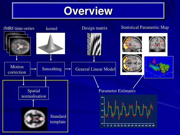
Statistical Parametric Map. Design matrix. fMRI time-series. kernel. Motion correction. Smoothing. General Linear Model. Spatial normalisation. Parameter Estimates. Standard template. Overview. The preprocessing sequence revisted. Realignment

E N D
Statistical Parametric Map Design matrix fMRI time-series kernel Motion correction Smoothing General Linear Model Spatial normalisation Parameter Estimates Standard template Overview
The preprocessing sequence revisted • Realignment • Motion correction: Adjust for movement between slices • Coregistration • Overlay structural and functional images: Link functional scans to anatomical scan • Normalisation • Warp images to fit to a standard template brain • Smoothing • To increase signal-to-noise ratio • Extras (optional) • Slice timing correction; unwarping
Co-registration • Term co-registration applies to any method for aligning images • By this token, motion correction is also co-registration • However, term is usually used to refer to alignment of images from different modalities. E.g.: • Low resolution T2* fMRI scan (EPI image) to high resolution, T1, structural image from the same individual
Co-registration: Principles behind this step of processing • When several images of the same participants have been acquired, it is useful to have them all in register • Image registration involves estimating a set of parameters describing a spatial transformation that ‘best ‘ matches the images together
fMRI to structural • Matching the functional image to the structural image • Overlaying activation on individual anatomy • Better spatial image for normalisation • Two significant differences between co-registering to structural scans and motion correction • When co-registering to structural, the images do not have the same signal intensity in the same areas; they cannot be subtracted • They may not be the same shape
Problem: Images are different • Differences in signal intensity between the images • Normalise to appropriate template (EPI to EPI; T1 to T1), then segment
Segmentation • Use the gray/white estimates from the normalisation step as starting estimates of the probability of each voxel being grey or white matter • Estimate the mean and variance of the gray/white matter signal intensities • Reassign probabilities for voxels on basis of • Probability map from template • Signal intensity and distributions of intensity for gray/white matter • Iterate until there is a good fit
Register segmented images • Grey/white/CSF probability images for EPI (T2*) and T1 • Combined least squares match (simultaneously) of gray/white/CSF images of EPI (T2*) + T1 segmented images
An alternative technique that relies on mutual information theory • Different material will have different intensities within a scan modality • E.g. air will have a consistent brightness, and this will differ from other materials (such as white matter)
From Bianca de Haan’s fmri guide. http://www.sph.sc.edu/comd/rorden/fmri_guide/
SPM co-registration - problems • Poor affine normalisation bad segmentation etc. • Image not homogeneous errors in clustering • Susceptibility holes in image (e.g. sinuses) errors in clustering/segmentation
The EPI scans can also be registered to subject’s own mean EPI image • Two images from the same subject acquired using the same modality generally look similar • Hence, it is sufficient to find the rigid-body transformation parameters that minimise the sum of squared differences between them • Easier than co-registration between modalities (intensity correspondence) • Can be spatially less precise • But more sensitive to detecting activity differences?
The preprocessing sequence revisted • Realignment • Motion correction: Adjust for movement between slices • Coregistration • Overlay structural and functional images: Link functional scans to anatomical scan • Normalisation • Warp images to fit to a standard template brain • Smoothing • To increase signal-to-noise ratio • Extras (optional) • Slice timing correction; unwarping
Normalisation Goal: Register images from different participants into roughly the same co-ordinate system (where the co-ordinate system is defined by a template image) • This enables: • Signal averaging across participants: • Derive group statistics -> generalise findings to population • Identify commonalities and differences between groups (e.g., patient vs. healthy) • Report results in standard co-ordinate system (e.g. Talairach and Tournoux stereotactic space)
Normalisation: Methods • Methods of registering images: • Label-based approaches: Label homologous features in source and reference images (points, lines, surfaces) and then warp (spatially transform) the images to align the landmarks (BUT: often features identified manually [time consuming and subjective!] and few identifiable landmarks) • Intensity-based approaches: Identify a spatial transformation that maximises some voxel-wise similarity measure (usually by minimising the sum of squared differences between images; BUT: assumes correspondence in image intensity [i.e., within-modality consistency], and susceptible to poor starting estimates) • Hybrid approaches – combine intensity method with user-defined features
SPM: Spatial Normalisation • SPM adopts a two-stage procedure to determine a transformation that minimises the sum of squared differences between images: • Step 1: Linear transformation (12-parameter affine) • Step 2: Non-linear transformation (warping) • High-dimensionality problem • The affine and warping transformations are constrained within an empirical Bayesian framework (i.e., using prior knowledge of the variability of head shape and size): “maximum a posteriori” (MAP)estimates of the registration parameters
Step 1: Affine Transformation Determines the optimum 12-parameter affine transformation to match the size and position of the images 12 parameters = 3 translations and 3 rotations (rigid-body) + 3 shears and 3 zooms Rotation Shear Translation Zoom
Step 2: Non-linear Registration • Assumes prior approximate registration with 12-parameter affine step • Modelled by linear combinations of smooth discrete cosine basis functions (3D) • Choice of basis functions depend on distribution of warps likely to be required • For speed and simplicity, uses a “small” number of parameters (~1000)
2-D visualisation (horizontal and vertical deformations): • Brain • visualisation: Ashburner; HBF Chap 3 Source Template Deformation field Warped image
Bayesian Framework • Using Bayes rule, we can constrain (“regularise”) the nonlinear fit by incorporating prior knowledge of the likely extent of deformations: • p(p|e) p(e|p) p(p) (Bayes Rule) • p(p|e)is the a posteriori probability of parameters p given errors e • p(e|p)is the likelihood of observing errors e given parameters p • p(p)is the a priori probability of parameters p • For maximum a posteriori (MAP) estimate, we minimise (taking logs): • H(p|e) H(e|p) + H(p) (Gibbs potential) • H(e|p)(-log p(e|p)) is the squared difference between the images (error) • H(p)(-log p(p)) constrains parameters (penalises unlikely deformations) • is “regularisation” hyperparameter, weighting effect of “priors” Rik Henson
Bayesian Constraints Empirically generated priors • Algorithm simultaneouslyminimises: • Sum of squared difference between template and source image (update weighting for each base) • Squared distance between the parameters and prior expectation (i.e., deviation of the transform from its expected value) • Bayesian constraints applied to both: 1) affine transformations • based on empirical prior ranges 2) nonlinear deformations • based on smoothness constraint (minimising membrane energy) Rik Henson
Template image Affine Registration (2 = 472.1) Non-linear registration with regularisation (2 = 302.7) Non-linear registration without regularisation (2 = 287.3) Bayesian Constraints Without the Bayesian formulation, the non-linear spatial normalisation can introduce unnecessary warping into the spatially normalised images
Normalisation: Caveats • Constrained to correct for only gross differences; residual variability is accommodated by subsequent spatial smoothing before analysis • Structural alignment doesn’t imply functional alignment • Differences in gyral anatomy and physiology between participants leads to non-perfect fit. Strict mapping to template may create non-existent features • Brain pathology may disrupt the normalisation procedure because matching susceptible to deviations from template image (-> can use brain masks for lesions, etc.; weight different regions differently so they have varied influence on the final solution) • Affine transforms not sufficient: Non-linear solutions are required • Optimally, move each voxel around until it fits. Millions of dimensions. • Trade off dimensionality against performance (potentially enormous number of parameters needed to describe the non-linear transformations that warp two images together; but much of the spatial variability can be captured with just a few parameters) • Regularization: use prior information (Bayesian scheme) about what fit is most likely (unlike rigid-body transformations where constraints are explicit, when using many parameters, regularization is necessary to ensure voxels remain close to their neighbours)
Normalisation: Solutions • Inspect images for distortions before transforming • Adjust image position before normalisation to reduce risk of local minima (i.e., best starting estimate) • Intensity differences: Consider matching to a local template • Image abnormalities: Cost-function masking
Sources: • Ashburner and Friston’s “Spatial Normalization Using Basis Functions” (Chapter 3, Human Brain Function, 2nd ed.; http://www.fil.ion.ucl.ac.uk/spm/doc/books/hbf2/) • Rik Henson’s Preprocessing Slides: • http://www.mrc-cbu.cam.ac.uk/Imaging/Common/rikSPM-preproc.ppt • Matthew Brett’s Spatial Processing Slides: • http://www.mrc-cbu.cam.ac.uk/Imaging/Common/Orsay/jb_spatial.pdf