Download
1 / 30
310 likes | 537 Views
ADAPTIVE CONTROL SYSTEMS. MRAC IV UNIT. BY Y.BHANUSREE ASST. PROFESSOR. MRAC. MODEL REFERENCE ADAPTIVE CONTROL SYSTEM It can be considered as an ADAPTIVE SERVO SYSTEM. It consists of two loops inner loop &outer loop

E N D
ADAPTIVE CONTROL SYSTEMS MRAC IV UNIT BY Y.BHANUSREE ASST. PROFESSOR
MRAC • MODEL REFERENCE ADAPTIVE CONTROL SYSTEM • It can be considered as an ADAPTIVE SERVO SYSTEM. • It consists of two loops inner loop &outer loop • It consists of a reference model in outer loop. • Ordinary feed back is called inner loop. • Parameters are adjusted on basis of feedback from the error. • Error is the difference between produced output & reference model value.
Adjustment of system parameters in a MRAC can be obtained in two ways. • GRADIENT METHOD (MIT RULE) • LYPNOV STABILITY THEORY
MODEL YM CONTROLLER PARAMETERS ADJUSTMENT MECHANISM UC U Y PLANT CONTROLLER BLOCK DIAGRAM OF MRAC
MRAC IS COMPOSED OF • Plant containing unknown parameters • Reference model • Adjustable parameters containing control law or loss law • Ordinary feed back loop
MIT RULE • It is developed by INSTRUMANTATION LABORATORY at MIT. • To consider MIT rule we use a closed loop response in which controller has one adjustable parameter θ. • The desired closed loop response is specified by a model whose output is ym. • Then error e= ym – y. (y is original output).
Error criteria selected here is • J(θ)=1/2 (e)2 • And this loss function is to be minimized to make the system controlled. • To achieve this the parameters are changed in the direction of negative gradient of J. • dθ = -γ∂J = - γe ∂e • dt dθ∂θ • This is called GRADIENT or MIT rule. • γ =adaptation gain • ∂e/ ∂θ = sensitivity derivative(informs how error is influenced by θ
The loss function can also be chosen as • J(θ)=|e| • dθ = - γ∂e sign e [GRADIENT METHOD] • dt ∂θ • first MRAC is implemented by this function • dθ = - γ sign ∂e sign (e) • dt ∂θ • [ sign-sign algorithm] • used in telecommunication where simple • implementation & fast computing are required
For multivariable systems • θ is considered as vector • ∂e/ ∂θ is considered as gradient of the error with respect to the parameter
APPLICATIONS FOR MIT RULE ADAPTATION OF A FEED FORWARD GAIN MRAS FOR A FIRST ORDER SYSTEM
ADAPTATION OF A FEED FORWARD GAIN PROBLEM :Adjustment of feed forward gain ASSUMPTIONS: • Process is linear with the transfer function KG(s) • G(s) is known • K is unknown parameter DESIRED CONDITION: Transfer function Gm(s) should be equal to KoG(s) Ko is given constant
MODEL Ym KOG(S) _ -γ/S e π ∑ + PROCESS θ U UC Y π KG(S) MRAC FOR ADJUSTMENT OF FEEDFORWARD GAIN BY MIT RULE
The constant k for this plant is unknown. However, a reference model can be formed with a desired value of k, and through adaptation of a feedforward gain, the response of the plant can be made to match this model. The reference model is therefore chosen as the plant multiplied by a desired constant ko . The cost function chosen here is,
The error is then restated in terms of the transfer functions multiplied by their inputs. As can be seen, this expression for the error contains the parameter theta which is to be updated. To determine the update rule, the sensitivity derivative is calculated and restated in terms of the model ouput:
Finally, the MIT rule is applied to give an expression for updating theta. The constants k and ko are combined into gamma. To tune this system, the values of ko and gamma can be varied.
NOTES ON DESIGN WITH MIT • It is important to note that the MIT rule by itself does not guarantee convergence or stability. • An MRAC designed using the MIT rule is very sensitive to the amplitudes of the signals. • As a general rule, the value of gamma is kept small. Tuning of gamma is crucial to the adaptation rate and stability of the controller.
IF G(S)=1/S+1 • UC is sinusoidal signal with frequency 1 rad/s • K=1 • K0=2 • Vary values of γ • γ=0.5,1,2 • We can observe the output approaches the model output at γ=1
OBSERVATIONS FROM GRAPH: • Convergence rate depends on adaptation gain γ. • Reasonable value of γ has to be selected . Applications: • In robots with unknown load. • CD player where sensitivity of laser diode is not known.
MRAC FOR A FIRST ORDER SYSTEM Processdy = −ay+bu dt Model dym = −amym+bmuc dt Controller U(t)=θ1Uc(t)- θ2 Y(t) θ1 & θ2 are 2 adjustable parameters
LYAPUNOV THEOREM ALGORITHM FOR LYAPUNOV THEORY • Derive differential equation for the error e=y-ym. • We attempt to find lyapunov function & an adaptation mechanism such that the error will go to zero. • We find dv/dt is usually only negative semi definite .so finding error equation & lyapunov function with a bounded second derivative . • It is to show bounded ness & that error goes to zero. • To show parameter convergence ,it is necessary to impose further conditions ,such as persistently excitation and uniform observability
MODEL YM KOG(S) e - UC θ ∑ -γ/S π + PROCESS Y KG(S) π B. DIAG FOR FEED FORWARD GAIN CONTROL USING LYAPUNOV RULE
The value of dv/dt is <=0 [which is –ve semi definite] • As time derivative of Lypanov function is negative semi definite. • By using lemma of lypanov we can show error goes to zero.
REFERENCES • http://www.control.hut.fi/Kurssit/AS-74.185/luennot/lu5ep.pdf • http://www.control.hut.fi/Kurssit/AS-74.185/luennot/lu6ep.pdf • http://www.control.lth.se/~FRT050/Exercises/ex4sol.pdf • http://www.control.lth.se/%7EFRT050/Exercises/ex5sol.pdf • http://www.igi.tugraz.at/helmut/Presentations/AdaptiveControl.html • http://www.irs.ctrl.titech.ac.jp/~dkura/ic2004/lec405.pdf • http://www.irs.ctrl.titech.ac.jp/~dkura/ic2004/lec406.pdf • http://mchlab.ee.nus.edu.sg/Experiment/Manuals/EE5140/adap1.pdf • http://www.rcf.usc.edu/~ioannou/RobustAdaptiveBook95pdf/Robust_Adaptive_Control.pdf