Download
1 / 37
420 likes | 712 Views
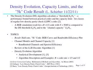
Density Evolution, Capacity Limits, and the "5k" Code Result (L. Schirber 11/22/11).

E N D
Density Evolution, Capacity Limits, and the "5k" Code Result (L. Schirber 11/22/11) The Density Evolution (DE) algorithm calculates a "threshold Eb/N0 " - a performance bound between practical codes and the capacity limit - for classes of regular low-density parity-check (LDPC) codes [2]. A BER simulation result for a R =1/2 code with N = 5040 is compared to the DE threshold Eb/N0 and to the “channel capacity” Eb/N0 . TOPICS Result: Half-rate, "5k" Code: BER Curve and Bandwidth-Efficiency Plot Channel Models and Channel Capacity [1] Bandlimited Channels and Spectral Efficiency Review of the LLR Decoder Algorithm [1] Density Evolution Algorithm Analytical Development [1], [3] Algorithm Description and Examples: R = code rate = 1/3 and 1/2 [1] Error Correction Coding: Mathematical Methods and Algorithms, by Moon (2005) [2]Gallager, "Low-Density Parity-Check Codes" , MIT Press (1963) [3] Barry, “Low-Density Parity-Check Codes”, Georgia Institute of Technology, (2001) Page 1 of 37
4-Cycle Removed vs Original LDPC Code: (N = 5040, M = 2520) Codes 2.7 million seconds = 31 days so the run for Eb/N0 = 1.75 dB took a CPU month on a PC! We try the 4-cycle removal algorithm (see Lecture 18) with a larger matrix. There is a slight improvement with 4-cycles removed, although there are only 11 word errors at BER = 1e-5. Note that in these cases every word error is a decoder failure (Nw = Nf ); hence there are no undetected codeword errors (Na1 = Na2 = 0). Page 2 of 37
N=1080 vs 5040 LDPC Codes : Gap to Capacity at a Given BER The half-rate, "5k" code is within about 1.6 dB at BER = 1e-5 of the Shannon limit Eb/N0 (magenta dash-dotted line). The Density Evolution (DE) threshold Eb/N0 (black dashed line)is also shown. Page 3 of 37
5k Code Result in the Bandwidth Efficiency Plane • BER performance is summarized by giving the required Eb/N0 to reach a certain BER level. • We choose a 10-5 BER level, and report a minimum Eb/N0 =1.75 dB necessary for that BER for the 5k code. • The "density evolution threshold" (red diamond) and the "capacity limit for a binary input AWGN channel" (green circle) are compared in the plot and table. Page 4 of 37
Channel Models and Channel Capacity BSC model 1 - p 0 0 p p 1 1 1 - p Y X Channel • We consider 3 “input X, output Y” channel models, • (1) the simple binary symmetric channel or BSC, • (2) the additive white Gaussian noise channel or AWGNC, and • (3) the binary-input AWGN channel or BAWGNC. • We calculate the mutual information function I(X;Y) from the definitions for each channel. • The resulting channel capacity C (from [1]), the maximum possible mutual information over all input distributions for X , is given and plotted versus a SNR measure. Page 5 of 37
Calculation of Channel Capacity C: Binary Symmetric Channel Example (1 of 5) • (b) By maximizing over q show that the channel capacity per channel use is • Exercise 1.31 (from [1]) For a BSC with crossover probability p having input X and output Y, let the probability of inputs be P(X = 0) = q and P(X = 1) = 1 - q. • (a) Show that the mutual information is Page 6 of 30
BSC model 1 - p 0 0 p p 1 1 1 - p Calculation of Channel Capacity: Binary Symmetric Channel Example (2 of 5) Page 7 of 37
Calculation of Channel Capacity: Binary Symmetric Channel Example (3 of 5)
Calculation of Channel Capacity: Binary Symmetric Channel Example (4 of 5)
BSC model 1 - p 0 0 p p 1 1 1 - p Calculation of Channel Capacity: Binary Symmetric Channel Example (5 of 5) Page 10 of 37
Calculation of Channel Capacity: Binary input AWGN Channel (BAWGNC) ( 1 of 3) • Example 1.10. Suppose we have a input alphabet Ax ={-a, a} (e.g., BPSK modulation with amplitude a) with P(X = a) = P(X = -a) = 1/2. Let N ~ N(0,2) and Y = X + N. Find the mutual information and channel capacity.
Calculation of Channel Capacity: Binary input AWGN Channel (BAWGNC) ( 2 of 3)
Calculation of Channel Capacity: Binary input AWGN Channel (BAWGNC) ( 3 of 3) Page 13 of 30
Aside: Probability Function f(y;a,1) • The probability function fis a function of y with two parameters: amplitude a and noise variance 2. We set 2 to 1 here for convenience. • f(y ;a, 2) is the average of two Gaussians – with separation 2a and common variance 2 - at a given y. • It has a shape resembling a Gaussian with variance s 2 for small SNR = a2/s 2, and two separated Gaussians with variance s 2 for large SNR. Page 14 of 37
Calculation of Channel Capacity: AWGN Channel • Example 1.11. Let X ~ N(0,x2)and N ~ N(0,n2) , independent of X. Let Y = X + N. Then Y ~ N(0,x2+ n2). Find the mutual information and capacity.
Capacity vs SNR for 3 Channel Models (from [1]) • Capacity (bits/channel use) is determined for the • Binary Symmetric Channel (BSC) • AWGN Channel (AWGNC) • Binary-input AWGN Channel (BAWGNC) Page 16 of 37
Bandlimited Channel Analysis: Capacity Rate • Assume that the channel is band-limited, i.e., the frequency content in any input, noise, or output signal is bounded above by frequency W in Hz. • By virtue of the Nyquist-Shannon Sampling theorem, then it is sufficient to choose a sampling frequency of 2W to adequately sample X, the channel input signal. • Recall that the channel has capacity C in units of bits or bits per channel use, which is the maximal mutual information between input X and output Y. • We can define a "capacity rate" - denoted here by C' to differentiate it from capacity C - in bit/s as the maximum possible rate of transfer of information for the bandlimited channel: • We define the spectral efficiency for a bandlimited channel as the ratio of the data rate (Rd) to W. The maximum spectral efficiency is equal to C'/W. Page 17 of 37
Aside: Shannon-Nyquist Sampling Theorem (from Wikipedia) • The Nyquist-Shannon (or Shannon-Nyquist) sampling theorem states: • Theorem: If a function s(t) contains no frequencies higher than W hertz, it is completely determined by giving its ordinates at a series of points spaced 1/(2W) seconds apart. • Suppose a continuous time signal s(t) is sampled at a finite number (Npts) of equally-spaced time values with sampling interval Dt . • In other words, we are given a “starting time” t0along with a sequence of values s[n] where s[n] = s(tn) for n = 1,2,…, Npts with tn = t0 + (n-1) Dt and where Dt = t2– t1. • If the signal is band-limited by W where W ≤ 1/(2Dt) , then the theorem says we can reconstruct the signal exactly: i.e., given the Npts values s[n] we can infer what the (continuous) function s(t) has to be for all t. Page 18 of 37
Spectral Efficiency Curve: Band-limited AWGN Channel Shannon limit “keep out” region • For a given Eb over N0 in dB, we find for the band-limited AWGN channel that there is a limiting value for spectral efficiency (measured in bit/second per hertz). • In other words, we cannot expect to transmit at a bit rate (Rd) greater than that times W, with W the channel bandwidth. • The Shannon limit is the minimum Eb / N0 for reliable communication. Page 19 of 37
Spectral Efficiency for AWGN, BAWGN, and Quaternary-input AWGN Channels Spectral Efficiency : Linear scale Spectral Efficiency : Log scale • The maximum spectral efficiencies () for AWGN, binary input AWGN, and quaternary input AWGN channels are shown above. For large Eb/N0 , goes to 1 (bit/s) / Hzfor the BAWGNC and 2 (bit/s) / Hz for the QAWGNC. • Next we work through the details of constructing these curves. Page 20 of 37
Procedure for Generating Spectral Efficiency vs SNR and Eb/N0 in dB Curves for Band-limited AWGN Channels • 6. Plot vs SNR and vs Eb/N0 in dB. • 1. Choose a range of (receiver) SNR, e.g., SNR= [.001: .01: 10]. • 2. Find the capacity C = f (SNR) in bits/channel use for each SNR. • 3. Determine the capacity bit rate C’ = 2WC in bit/s, where the channel is used 2W times per second, W the channel bandwidth, and = 1 for AWGNC or QAWGNC, 1/2 for QAWGNC. • 4. Calculate the max spectral efficiency = C’/W with units of (bit/s)/Hz. • 5. For each SNR also determine the corresponding (received) Eb/N0 in dB: Page 21 of 37
Generating Spectral Efficiency Curves, Example 2: Band-limited, Binary-input AWGN Channel plot of (SNR) for 0 < SNR < 10 plot of (Eb /N0) with Eb /N0 in dB Page 22 of 37
Message Passing Formulas in the LLR Decoder Algorithm j cj, j in Nm',n' . . . . . . tier 2 zm' , m' in Mn',m . . . tier 1 checks m',n' cn' , n' in Nm,n tier 1 zm , m in Mn root checks (3,6) Code: Parity Check Tree from Bit cn root cn • The LLR decoder computes check LLRs from bit LLRs, and then bit LLRs from check LLRs. • Assume that (cj | r) is approximately equal to (cj | r\n) for j n. • We can visualize these computations as passing LLRs along edges of the Parity Check graph. Page 23 of 30
adjustment to remove intrinsic information LLR LDPC Decoder Algorithm [2] Page 24 of 37
Ground Rules and Assumptions for Density Evolution • Density evolution tracks the iteration-to-iteration PDFs calculated in the log likelihood ratio (LLR) LDPC decoder algorithm (using BPSK over AWGN). • The analysis presented here makes several simplifying assumptions: • 1. The code is regular with wc = column weight, wr = row weight, and the code length N is very large. • 2. The Tanner graph is a tree, or no cycles exist in the graph. • 3. The all-zero codeword is sent, so the received vector is Gaussian. • 4. The bit and check LLRs - the n for 1 n N and m,n for 1 m Mand 1 n N - are consistent random variables, and are identically distributed over n and m. • The means of the check LLRs - denoted by [l] for the mean at iteration l - satisfy a recurrence relation, which is described next.
Density Evolution Analysis (1 of 6) De-Mapper and Decoder A, L m c t r + Rd = 1 bit/s Tb = 1/Rd = 1s = bit time a Encoder R = K/N, A, G Signal Mapper (e.g., BPSK) • Vector r is assumed to be equal to the mapped codeword plus random noise from the channel (i.e., ideal synchronization and detection are assumed). • Here we assume the channel is AWGN, so each component of the noise is a (uncorrelated) Gaussian random variable with zero mean and known variance 2 (found from a, the code rate R, and ratio Eb / N0 ) Suppose we map 0 to a and 1 to -a, with a denoting a signal amplitude for a (baseband BPSK) transmitted waveform, (over an assumed 1 ohm load). Page 26 of 37
Density Evolution Analysis (2 of 6) Signal Mapper (e.g., BPSK) De-Mapper and Decoder A, L m = 0 t r c = 0 Encoder R = K/N, A, G + a Rd = 1 bit/s Tb = 1/Rd = 1s = bit time • The PDF for rn with this all-zero codeword assumption is Gaussian, with the same mean and variance for each n: Suppose (without loss of generality) that the all-zero codeword is transmitted, which implies for our current definitions that tn= a for n = 1,2, …, N.
Density Evolution Analysis (3 of 6) • Hence we see that the initial bit LLRs are all Gaussian, each with variances equal to twice their means. We call these random variables consistent . • Although the initial PDFs of the bit LLRs are consistent, subsequent iterations are not in general; however, we assume that all bit LLR PDFs are consistent. • Also assume that the nare identically distributed over n: i.e., the means of the bit LLRs or m[l] are the same for each n, but do vary with iteration l. Recall that the LLR decoder algorithm (Algorithm 15.2) initializes bit LLRs or bit “messages” – the (cn | r) or n- to a constant (Lc) times rn. Page 28 of 37
Aside: Consistent Random Variables • For density evolution we assume that the bit and check LLRs are consistent random variables. Furthermore, their statistics depend only on iteration number (l), not on (indices) m or n. • If the mean of the LLR increases towards infinity, the corresponding bit (or check) estimate becomes more certain. • Define a random variable to be consistent if: • 1. it is Gaussian, and • 2. its variance is equal to twice its mean in absolute value: Page 29 of 37
Density Evolution Analysis (4 of 6) • Furthermore, assume the check LLRs are consistent and identically distributed. • Assume the LDPC code is (wc ,wr)-regular, and the Tanner graph is cycle-free. • The bits (cj) in check m besides n will be distinct – by the cycle-free assumption - and assuming they are also conditionally independent on r\n allows us to use the tanh rule to relate the bit LLRs and check LLRs: Page 30 of 37
Density Evolution Analysis (5 of 6) • Take the expectation of both sides of (8). • Define a function (x) as below, plotted on the right along with tanh(x/2). Recast (9) in terms of (x) to write down (10). Page 31 of 37
Aside: Function Y(x) and Inverse x = -1(y), -1 < y < 1 y = (x), for any x, … but only -10 < x < 10 shown We will need to evaluate the bounded function Y(x) , where x is any real number and y ranges between -1 to 1. The inverse function also needs to be evaluated, and its evaluation (near y = 1 or -1) leads to numerical instabilities. Page 32 of 37
Density Evolution Analysis (6 of 6) • From the bit LLR update equation in the LLR decoding algorithm (with some re-shuffling of operations). • Take the expected value of both sides of (11). • Plug (12) into (10) to develop (13), a recurrence relation for sequence [l]. Initialize the calculations with [l]= 0 for l = 0. Page 33 of 37
Density Evolution Algorithm Page 34 of 37
Density Evolution: Example 1 (Example 15.8 in[1] ) Eb/N0 = 1.8 dB, max = 100 max after ~55 iters Eb /N0 = 1.76 dB, max = 100 0.381 Eb/N0 = 1.764 dB, max = 100 max after ~550 iters • note: LLR = 30 • P(zm,n = 0) > 1-10-12 • cn = 0 for all n • Check LLR mean value approaches a constant if Eb/N0 is less than the threshold {Eb/N0}t , or approaches infinity if Eb/N0 > {Eb/N0}t . Here {Eb/N0}t 1.764 dB. Page 35 of 37
Density Evolution: Example 2 Eb/N0 = 1.2 dB, max = 100 max after ~128 iters Eb /N0 = 1.16 dB, max = 100 0.785 Eb/N0 = 1.19 dB, max = 100 0.945 • Here {Eb/N0}t 1.2 dB. Page 36 of 37
Comparing Density Evolution Results (from [4]) : Comparisons to [1], p 659 • 3 Density Evolution cases were attempted; the thresholds produced are listed in red. • Apparently, there is a slight (<.05 dB) discrepancy between Moon's results (taken from [4]) in Table 15.1 and mine. • However, his Example 15.8 and Figure 15.11 suggest a threshold of 1.76, not 1.73 for the R = 1/3 rate case. Page 37 of 37 [4] "Analysis of Sum-Product Decoding of Low-Density Parity-Check Codes Using a Gaussian Approximation", by Chung, Richardson, and Urbanke, IEEE Transactions in Information Theory, vol. 47, no. 2, (2001)