Download
1 / 13
130 likes | 234 Views
Constraining Astronomical Populations with Truncated Data Sets. Brandon C. Kelly (CfA, Hubble Fellow, bckelly@cfa.harvard.edu). Goal of Many Surveys: Understand the distribution and evolution of astronomical populations. How does the growth of supermassive black holes change over time?

E N D
Constraining Astronomical Populations with Truncated Data Sets Brandon C. Kelly (CfA, Hubble Fellow, bckelly@cfa.harvard.edu) Brandon C. Kelly, bckelly@cfa.harvard.edu
Goal of Many Surveys: Understand the distribution and evolution of astronomical populations • How does the growth of supermassive black holes change over time? • How was the stellar mass of galaxies assembled? • What is the distribution of black hole spin for supermassive black holes? How does this evolve? But all we can observe (measure) is the light (flux density) and location of sources on the sky! Brandon C. Kelly, bckelly@cfa.harvard.edu
A motivating example • Recent advances in modeling of stellar evolution have made it possible to relate a galaxy’s physical parameters (e.g., mass, star formation history) to its measured fluxes • Opens up possibility of studying evolution of galaxy population, and, in particular, evolution in the distribution of their physical quantities, and not just their measurable ones. Brandon C. Kelly, bckelly@cfa.harvard.edu
Simple vs. Advanced Approach Simple but not Self-consistent Advanced and Self-Consistent Derive distribution and evolution of quantities of interest directly from observed distribution of measurable quantities Circumvents fitting of individual sources independently Self-consistently accounts for uncertainty in derived quantities and selection effects (e.g., flux limit) • Derive ‘best-fit’ estimates for quantities of interest (e.g., mass, age, BH spin) • Do this individually for each source • Infer distribution and evolution directly from the estimates • Provides a biased estimate of distribution and evolution Brandon C. Kelly, bckelly@cfa.harvard.edu
The Posterior Distribution: How to quantitatively relate the distribution of physical quantities to measurable ones • Define p(y|x) as the measurement model, it relates the physical quantities, x, to the measured ones, y • Define p(x|θ) as the model distribution for the physical quantities • The posterior probability distribution of the values of x (physical quantities) and θ (parameterizes distribution of x), given the values of y (measured quantities) for the n data points: Brandon C. Kelly, bckelly@cfa.harvard.edu
Incorporating the flux limit (truncation) • If there is a flux limit (data truncation), denote Det(y) to be the selection function (probability of detection as a function of y). We need to normalize the posterior by the detection probability as a function of θ, Det(θ): • The probability distribution of the physical (missing) quantities for each source, x, and the parameters for the distribution of x, θ, given the n observed values of y, is then Brandon C. Kelly, bckelly@cfa.harvard.edu
But, there are some computational complications… • Expected fluxes are a highly non-linear, non-monotonic function of the physical parameters • Leads to multiple modes in p(y|x), and thus in the posterior • Calculation of expected flux for a given physical parameter set is very computationally intensive, based on running a complex computer model for stellar evolution • Typical to run model on a grid first, and then use a look-up table Brandon C. Kelly, bckelly@cfa.harvard.edu
Example Posterior Probability Distribution Brandon C. Kelly, bckelly@cfa.harvard.edu
Additional problems when there is truncation (e.g., a flux limit) • No simple way to calculate Det(θ): • Naïve method: Simulate a sample given the model, θ, and count the fraction of sources that are detected • Unfortunately, this stochastic integral introduces error in Det(θ), and posterior is unstable to even small errors in Det(θ) Brandon C. Kelly, bckelly@cfa.harvard.edu
Example: Estimating a Luminosity Function (Distribution) • Simulate galaxy luminosities from a Schechter function (i.e., a gamma distribution) • Keep L > LLIM = L* (~ 30% detection fraction) • Estimate Det(α,L*) stochastically: • For each (α,L*) simulate a sample of 1000 and 10,000 luminosities • Keep those for which L > LLIM Brandon C. Kelly, bckelly@cfa.harvard.edu
Statistical and computational problems, and directions for future work • Need to have more efficient algorithms • Modern and future surveys will produce tens to hundreds of thousands of data points with several parameters (e.g., flux densities) each, how to efficiently do statistical inference (e.g., MCMC)? • Potential algorithms need to handle multimodality in the posterior/likelihood function • Need to efficiently and accurately compute the multi-dimensional integral for the detection probability • Alternatively, need to efficiently account for uncertainty in a more efficient but less accurate integration method, e.g., stochastic integration • Need to have an accurate and efficient method for interpolating the output from computationally intensive computer models (e.g., stellar evolution) • Statistical emulators should help here Brandon C. Kelly, bckelly@cfa.harvard.edu
Example: The Quasar Black Hole Mass Function (Distribution) Intrinsic Distribution Of Derived Quantities Intrinsic Distribution of Measurables Selection Effects Observed Distribution of Measurables Black Hole Mass Luminosity Luminosity Emission Line Width Emission Line Width Flux Limit Eddington Ratio Brandon C. Kelly, bckelly@cfa.harvard.edu
Example on Real Data: The Quasar Black Hole Mass Function (Distribution) From Kelly et al. (2010, ApJ, 719, 1315) Brandon C. Kelly, bckelly@cfa.harvard.edu