Download
1 / 20
200 likes | 282 Views
This academic paper compares beliefs and surveys in 3-SAT problems, focusing on Weighted SAT (WSAT) and Survey Propagation (SP) methods. The study explores the depth of decimation achieved and the impact of various strategies on formula complexity.

E N D
Comparing Beliefs, Surveys, and Random Walks for 3-SAT Scott Kirkpatrick, Hebrew University Joint work with Erik Aurell and Uri Gordon (see cond-mat/0406217 v1 9 June 2004)
Main Results • Rederive SP as a special case of BP • Permits interesting generalizations • Visualize decimation guided by SP as a flow • Study the depth of decimation achieved • WSAT as a measure of formula complexity • Depends on details of “tricks” employed • Shows SP produces renormalization out of hard-SAT • With today’s codes, WSAT outperforms SP! • Except in regime where 1-RSB is stable • WSAT has an endpoint at 4.15
Beliefs and Surveys: • BP: evaluate the probability that variable x is TRUE in a solution • SP: evaluate the probability that variable x is TRUE in all solutions • This leaves a third case, x is “free” to be sometimes TRUE sometimes FALSE
Transports and Influences • To calculate the beliefs, or the slightly more complicated surveys, we introduce quantities associated with the directed links of the hypergraph: • (transport) T(ia) = fraction of solutions s.t. variable i satisfies clause a • (influence) I(ai) = fraction of solutions s.t. clause a is satisfied by variables other than I • I(ai) T(ja) + T(ka) – T(ja)T(ka) • Same iteration for BP, SP
Closing the loop introduces a one parameter family of belief schemes • Calculate new T’s from the I’s, and normalize… • (PPT is equation-challenged – do this on the board) • Iterative equations for SP differ from BP in one term • Interpolation formula seems useful in between: • Rho = 0 BP • Rho = 1 SP • 0 < Rho < 1 BP SP • 1 < Rho SP unknown • Interpret effects of Rho in flow diagram:
Visualize decimation as flows in the SP space Decimate variables closest to the corners Origin is the “paramagnetic phase”
BP, SP, hybrids differ in their “depth of decimation” These results are for SP only
What is accomplished by decimation? • A form of renormalization transform • Simplify the formula by eliminating variables, moving out of the hard-SAT regime • 3.92 < alpha < 4.267 • We use WSAT (from H. Kautz, B. Selman, B. Cohen) as a standard measure of complexity
Results of SP + decimation: Upper curves: WSAT cost/spin Lower curves: WSAT cost/spin after decimation (two normalizations)
Where does this pay off? • Using today’s programs, with local updates to recalculate surveys after each decimation step • N = 10,000, alpha = 4.1, 100 formulas • WSAT only 9.2 sec each • WSAT after decimation 0.3 sec each • But SP cost 62 sec each • N = 10,000, alpha = 4.2, 100 formulas • WSAT only 278 sec each • WSAT after decimation 3 sec each • SP cost 101 sec each
Investigate WSAT more carefully • WSAT evolved by trial and error, not subject to any “physical” prejudices or intuitions • Central trick is to always choose an unsat clause at random • Totally focussed on “break count” – number of sat clauses which depend on the spin chosen, become unsat • WSAT has one trick not included in the Weigt, Monasson studies: • Always check first for “free” moves, those with zero breakcount • If no free moves, then take random or greedy move with equal probability
WSAT cost/spin variance shrinks with N Examination of distributions shows that cost/spin is concentrated as N infty up to alpha = 4.15!
Conclusions • SP a special case of BP • Permits interesting generalizations • Visualize decimation guided by SP as a flow • Study the depth of decimation achieved • WSAT as a measure of formula complexity • Depends on details of “tricks” employed • Shows SP produces renormalization out of hard-SAT • With today’s codes, WSAT outperforms SP! • Except in regime where 1-RSB is stable • WSAT has an endpoint at 4.15