Download
1 / 33
330 likes | 571 Views
Synchronous Control and State Machines in Modelica. Hilding Elmqvist Dassault Systèmes Sven Erik Mattsson , Fabien Gaucher, Francois Dupont Dassault Systèmes Martin Otter, Bernhard Thiele DLR. Content. Introduction Synchronous Features of Modelica Synchronous Operators

E N D
Synchronous Control and State Machines in Modelica Hilding Elmqvist Dassault Systèmes Sven Erik Mattsson, Fabien Gaucher, Francois Dupont Dassault Systèmes Martin Otter, Bernhard Thiele DLR
Content • Introduction • Synchronous Features of Modelica • Synchronous Operators • Base-clock and Sub-clock Partitioning • Modelica_Synchronous library • State Machines • Conclusions
Introduction model Asynchronous_Modelica33 Real x(start=0,fixed=true), y(start=0,fixed=true), z; equation when Clock(0.33) then x = previous(x)+1; end when; when Clock(1,3) then y = previous(y)+1; end when; z = x-y; end Asynchronous_Modelica33; model Asynchronous_Modelica32 Real x(start=0,fixed=true), y(start=0,fixed=true), z; equation when sample(0,0.33) then x = pre(x)+1; end when; when sample(0,1/3) then y = pre(y)+1; end when; z = x-y; end Asynchronous_Modelica32; • Why synchronous features in Modelica 3.3? Rationalnumber 1/3 x and y must have the same clock Implicit hold z = x-y • Error Diagnostics for safer systems!
Introduction • Scope of Modelica extended • Covers complete system descriptions including controllers • Clocked semantics • Clock associated with variable type and inferred • For increased correctness • Based on ideas from Lucid Synchrone and other synchronous languages • Extended with multi-rate periodic clocks, varying interval clocks and Boolean clocks
Synchronous Features of Modelica • Plant and Controller Partitioning • Boundaries between continuous-time and discrete-time equations defined by operators. • sample(): samples a continuous-time variable and returns a clocked discrete-time expression • hold(): converts from clocked discrete-time to continuous-time by holding the value between clock ticks • sample operator may take a Clock argument to define when sampling should occur
Mass with Spring Damper • Consider a continuous-timemodel partial model MassWithSpringDamper parameter Modelica.SIunits.Mass m=1; parameter Modelica.SIunits.TranslationalSpringConstant k=1; parameter Modelica.SIunits.TranslationalDampingConstant d=0.1; Modelica.SIunits.Position x(start=1,fixed=true) "Position"; Modelica.SIunits.Velocity v(start=0,fixed=true) "Velocity"; Modelica.SIunits.Force f "Force"; equation der(x) = v; m*der(v) = f - k*x - d*v; end MassWithSpringDamper;
Synchronous Controller • Discrete-time controller model SpeedControl extends MassWithSpringDamper; parameter Real K = 20 "Gain of speed P controller"; parameter Modelica.SIunits.Velocityvref = 100 "Speed ref."; discrete Real vd; discrete Real u(start=0); equation // speed sensor vd = sample(v, Clock(0.01)); // P controller for speed u = K*(vref-vd); // force actuator f = hold(u); end SpeedControl; Samplecontinuousvelocity v with periodic Clock with period=0.01 The clock of the equationis inferred to be the same as for the variable vd which is the result of sample() Holddiscrete variable u betweenclock ticks
Discrete-time State Variables • Operator previous() is used to access the value at the previousclock tick (cf pre() in Modelica 3.2) • Introducesdiscretestate variable • Initial valueneeded • interval() is used to inquire the actual interval of a clock
Base-clocks and Sub-clocks • A Modelica model will typically have several controllers for different parts of the plant. • Such controllers might not need synchronization and can have different base clocks. • Equations belonging to different base clocks can be implemented by asynchronous tasks of the used operating system. • It is also possible to introduce sub-clocks that tick a certain factor slower than the base clock. • Such sub-clocks are perfectly synchronized with the base clock, i.e. the definitions and uses of a variable are sorted in such a way that when sub-clocks are activated at the same clock tick, then the definition is evaluated before all the uses. • New base type, Clock: ClockcControl = Clock(0.01); ClockcOuter =subSample(cControl, 5);
Sub and super sampling and phase modelSynchronousOperators Real u; Realsub; Realsuper; Realshift(start=0.5); Realback; equation u = sample(time, Clock(0.1)); sub =subSample(u, 4); super =superSample(sub, 2); shift =shiftSample(u, 2, 3); back =backSample(shift, 1, 3); end SynchronousOperators;
ExactPeriodic Clocks • Clocks defined by Real number period are not synchronized: Clock c1 = Clock(0.1); Clock c2 =superSample(c1,3); Clock c3 = Clock(0.1/3); // Not synchronized with c2 • Clocks defined by rationalnumber period are synchronized: Clock c1 = Clock(1,10); // period = 1/10 Clock c2 =superSample(c1,3); // period = 1/30 Clock c3 = Clock(1,30); // period = 1/30
Modelica_Synchronous library • Synchronous language elements of Modelica 3.3are “low level”: • Modelica_Synchronous library developed to access language elements in a convenient way graphically: // speed sensor vd = sample(v, Clock(0.01)); // P controller for speed u = K*(vref-vd); // force actuator f = hold(u);
Blocks that generate clock signals Generates a periodic clock with a Real period parameter Modelica.SIunits.Time period; ClockOutput y; equation y = Clock(period); Generates a periodic clock as an integer multipleof a resolution (defined by an enumeration). Code for 20 ms period: • y =superSample(Clock(20), 1000); super-sample clock with 1000 Clock with period 20 s period = 20 / 1000 = 20 ms Generates an event clock: The clock ticks whenever the continuous-time Boolean input changes from false to true. • y =Clock(u);
Sample and Hold Holds a clocked signal and generates a continuous-time signal. Before the first clock tick, the continuous-time output y is set to parameter y_start Discrete-time PI controller • y =hold(u); Purely algebraic block fromModelica.Blocks.Math Samples a continuous-time signaland generates a clocked signal. • y =sample(u); • y =sample(u, clock);
Sub- and Super-Sampling Defines that the output signal is an integer factor faster as the input signal, using a “hold” semantics for the signal. By default, this factor is inferred. It can also be defined explicitly. • y =superSample(u);
Defines that the output signal is an integer factor slower as the input signal, picking every n-th value of the input. • y =subSample(u,factor);
Varying Interval Clocks • The first argument of Clock(ticks, resolution) may be time dependent • Resolution must not be time dependent • Allowingvarying interval clocks • Can be sub and super sampled and phased modelVaryingClock IntegernextInterval(start=1); Clock c = Clock(nextInterval, 100); Real v(start=0.2); equation when c then nextInterval = previous(nextInterval) + 1; v = previous(v) + 1; end when; end VaryingClock;
Boolean Clocks • Possible to define clocks that tick when a Boolean expression changes from false to true. • Assume that a clock shall tick whenever the shaft of a drive train passes 180o. modelBooleanClock Modelica.SIunits.Angle angle(start=0,fixed=true); Modelica.SIunits.AngularVelocity w(start=0,fixed=true); Modelica.SIunits.Torque tau=10; parameter Modelica.SIunits.Inertia J=1; Modelica.SIunits.Angle offset; equation w =der(angle); J*der(w) = tau; when Clock(angle >= hold(offset)+Modelica.Constants.pi) then offset = sample(angle); end when; end BooleanClock;
DiscretizedContinuous Time • Possible to convertcontinuous-time partitions to discrete-time • A powerful feature since in many cases it is no longer necessary to manually implement discrete-time components • Build-up a inverse plant model or controller with continuous-time components and then sample the input signals and hold the output signals. • And associate a solverMethod with the Clock. modelDiscretized Real x1(start=0,fixed=true); Real x2(start=0,fixed=true); equation der(x1) = -x1 + 1; der(x2) = -x2 + sample(1, Clock(Clock(0.5), solverMethod="ExplicitEuler")); end Discretized;
State Machines • Modelica extended to allow modeling of control systems • Any block without continuous-time equations or algorithms can be a state of a state machine. • Transitions between such blocks are represented by a new kind of connections associated with transition conditions. • The complete semantics is described using only 13 Modelica equations. • A cluster of block instances at the same hierarchical level which are coupled by transition equations constitutes a state machine. • All parts of a state machine must have the same clock. (We will work on removing this restriction ,allowing mixing clocks and allowing continuous equations, in future Modelica versions.) • One and only one instance in each state machine must be marked as initial by appearing in an initialState equation.
A Simple State Machine inner i outer output i outer output i
A Simple State Machine – Modelica Text Representation model StateMachine1 inner Integeri(start=0); block State1 outer output Integeri; equation i = previous(i) + 2; end State1; State1state1; block State2 outer output Integeri; equation i = previous(i) - 1; end State2; State2state2; equation initialState(state1); transition(state1, state2, i > 10, immediate=false); transition(state2, state1, i < 1, immediate=false); end StateMachine1;
Merging Variable Definitions • An outer output declaration means that the equations have access to the corresponding variable declared inner. • Needed to maintain the single assignment rule. • Multiple definitions of such outer variables in different mutually exclusive states of one state machine need to be merged. • In each state, the outer output variables (vj) are solved for (exprj) and, for each such variable, a single definition is automatically formed: • v := ifactiveState(state1) then expr1elseifactiveState(state2) then expr2elseif … else last(v) • last() is a special internal semantic operator returning its input. It is just used to mark for the sorting that the incidence of its argument should be ignored. • A start value must be given to the variable if not assigned in the initial state. • Such a newly created assignment equation might be merged on higher levels in nested state machines.
Defining a State machine transition(from, to, condition, immediate, reset, synchronize, priority) • This operator defines a transition from instance “from” to instance “to”. The “from” and “to” instances become states of a state machine. • The transition fires when condition = true if immediate = true (this is called an “immediate transition”) or previous(condition) when immediate = false (this is called a “delayed transition”). • If reset = true, the states of the target state are reinitialized, i.e. state machines are restarted in initial state and state variables are reset to their start values. • If synchronize = true, the transition is disabled until all state machines within the from-state have reached the final states, i.e. states without outgoing transitions. • “from” and “to” are block instances and “condition” is a Boolean expression. • “immediate”, “reset”, and “synchronize” (optional) are of type Boolean, have parametric variability and a default of true, true, false respectively. • “priority” (optional) is of type Integer, has parametric variability and a default of 1 (highest priority). Defines the priority of firing when several transitions could fire. initialState(state) • The argument “state” is the block instance that is defined to be the initial state of a state machine.
Conditional Data Flows • Alternative to using outer output variables is to use conditional data flows. block Increment extends Modelica.Blocks.Interfaces.PartialIntegerSISO; parameter Integer increment; equation y = u + increment; end Increment; blockPrev extends Modelica.Blocks.Interfaces.PartialIntegerSISO; equation y = previous(u); end Prev; protectedconnector (node) i
Merge of Conditional Data Flows • It is possible to connect several outputs to inputs if all the outputs come from states of the same state machine. u1 = u2 = … = y1 = y2 = … with ui inputs and yi outputs. • Let variable v represent the signal flow and rewrite the equation above as a set of equations for ui and a set of assignment equations for v: • v := ifactiveState(state1) then y1else last(v);v := ifactiveState(state2) then y2else last(v);…u1 = vu2 = v… • The merge of the definitions of v is then made as described previously: v = ifactiveState(state1) then y1 elseifactiveState(state2) then y2elseif … else last(v)…
Hierarchical State Machine Example • stateA declares v as ‘outer output’. • state1 is on an intermediate level and declares v as ‘inner outer output’, i.e. matches lower level outer v by being inner and also matches higher level inner v by being outer. • The top level declares v as inner and gives the start value.
Reset and Synchronize • count is defined with a start value in state1. It is reset when a reset transition (v>=20) is made to state1. • stateY declares a local counter j. It is reset at start and as a consequence of the reset transition (v>=20) from state2 to state1. • The reset of j is deferred until stateY is entered by transition (stateX.i>20) although this transition is not a reset transition. • Synchronizing the exit from the two parallel state machines of state1 is done by using a synchronized transition.
Acausal Models in States – Modelica 3.3+ • The equations of each state is guarded by the activity condition • Should time variable be stopped when not active? • Should time be reset locally in state by a reset transition? • Special Boolean operator exception() to detect a problem in one model and transition to another model
Multiple Acasual Connections // C_p_i+brokenDiode_n_i+diode_n_i+load_p_i = 0.0; Replaced by: C_p_i + (if activeState(brokenDiode) then brokenDiode_n_i else 0) + (if activeState(diode) then diode_n_i else 0) + load_p_i = 0.0;
Conclusions • We have introduced synchronous features in Modelica 3.3. • For a discrete-time variable, its clock is associated with the variable type and inferencing is supported. • Special operators have to be used to convert between clocks. • This gives an additional safety since correct synchronization is guaranteed by the compiler. • We have described how state machines can be modeled in Modelica 3.3. • Instances of blocks connected by transitions with one such block marked as an initial state constitute a state machine. • Hierarchical state machines can be defined with reset or resume semantics, when re-entering a previously executed state. • Parallel sub-state machines can be synchronized when they reached their final states. • Special merge semantics have been defined for multiple outer output definitions in mutually exclusive states as well as conditional data flows.