Download
1 / 43
430 likes | 458 Views
Learn about rasterization strategies, clipping algorithms, hidden-surface removal, and more in computer graphics. Explore Cohen-Sutherland and Liang-Barsky algorithms for efficient polygon clipping.

E N D
Computer Graphics- Rasterization - Hanyang University Jong-Il Park
Objectives • Introduce basic rasterization strategies • Clipping • Scan conversion • Introduce clipping algorithms for polygons • Survey hidden-surface algorithms
Overview • At end of the geometric pipeline, vertices have been assembled into primitives • Must clip out primitives that are outside the view frustum • Algorithms based on representing primitives by lists of vertices • Must find which pixels can be affected by each primitive • Fragment generation • Rasterization or scan conversion
Required Tasks • Clipping • Rasterization or scan conversion • Transformations • Some tasks deferred until fragement processing • Hidden surface removal • Antialiasing
Rasterization Meta Algorithms • Consider two approaches to rendering a scene with opaque objects • For every pixel, determine which object that projects on the pixel is closest to the viewer and compute the shade of this pixel • Ray tracing paradigm • For every object, determine which pixels it covers and shade these pixels • Pipeline approach • Must keep track of depths
Clipping • 2D against clipping window • 3D against clipping volume • Easy for line segments and polygons • Hard for curves and text • Convert to lines and polygons first
Clipping 2D Line Segments • Brute force approach: compute intersections with all sides of clipping window • Inefficient: one division per intersection
Cohen-Sutherland Algorithm • Idea: eliminate as many cases as possible without computing intersections • Start with four lines that determine the sides of the clipping window y = ymax x = xmin x = xmax y = ymin
The Cases • Case 1: both endpoints of line segment inside all four lines • Draw (accept) line segment as is • Case 2: both endpoints outside all lines and on same side of a line • Discard (reject) the line segment y = ymax x = xmin x = xmax y = ymin
The Cases • Case 3: One endpoint inside, one outside • Must do at least one intersection • Case 4: Both outside • May have part inside • Must do at least one intersection y = ymax x = xmin x = xmax
Defining Outcodes • For each endpoint, define an outcode • Outcodes divide space into 9 regions • Computation of outcode requires at most 4 subtractions b0b1b2b3 b0 = 1 if y > ymax, 0 otherwise b1 = 1 if y < ymin, 0 otherwise b2 = 1 if x > xmax, 0 otherwise b3 = 1 if x < xmin, 0 otherwise
Using Outcodes • Consider the 5 cases below • AB: outcode(A) = outcode(B) = 0 • Accept line segment
Using Outcodes • CD: outcode (C) = 0, outcode(D) 0 • Compute intersection • Location of 1 in outcode(D) determines which edge to intersect with • Note if there were a segment from A to a point in a region with 2 ones in outcode, we might have to do two intersections
Using Outcodes • EF: outcode(E) logically ANDed with outcode(F) (bitwise) 0 • Both outcodes have a 1 bit in the same place • Line segment is outside of corresponding side of clipping window • reject
Using Outcodes • GH and IJ: same outcodes, neither zero but logical AND yields zero • Shorten line segment by intersecting with one of sides of window • Compute outcode of intersection (new endpoint of shortened line segment) • Reexecute algorithm
Efficiency • In many applications, the clipping window is small relative to the size of the entire data base • Most line segments are outside one or more side of the window and can be eliminated based on their outcodes • Inefficiency when code has to be reexecuted for line segments that must be shortened in more than one step
Cohen Sutherland in 3D • Use 6-bit outcodes • When needed, clip line segment against planes
Liang-Barsky Clipping • Consider the parametric form of a line segment • We can distinguish between the cases by looking at the ordering of the values of a where the line determined by the line segment crosses the lines that determine the window p(a) = (1-a)p1+ ap2 1 a 0 p2 p1
Liang-Barsky Clipping • In (a): a4 > a3 > a2 > a1 • Intersect right, top, left, bottom: shorten • In (b): a4 > a2 > a3 > a1 • Intersect right, left, top, bottom: reject
Advantages • Can accept/reject as easily as with Cohen-Sutherland • Using values of a, we do not have to use algorithm recursively as with C-S • Extends to 3D
Polygon Clipping • Not as simple as line segment clipping • Clipping a line segment yields at most one line segment • Clipping a polygon can yield multiple polygons • However, clipping a convex polygon can yield at most one other polygon
Tessellation and Convexity • One strategy is to replace nonconvex (concave) polygons with a set of triangular polygons (a tessellation) • Also makes fill easier • Tessellation code in GLU library
Clipping as a Black Box • Can consider line segment clipping as a process that takes in two vertices and produces either no vertices or the vertices of a clipped line segment
Pipeline Clipping of Line Segments • Clipping against each side of window is independent of other sides • Can use four independent clippers in a pipeline
Pipeline Clipping of Polygons • Three dimensions: add front and back clippers • Strategy used in SGI Geometry Engine • Small increase in latency
Bounding Boxes • Rather than doing clipping on a complex polygon, we can use an axis-aligned bounding box or extent • Smallest rectangle aligned with axes that encloses the polygon • Simple to compute: max and min of x and y
Bounding boxes Can usually determine accept/reject based only on bounding box reject accept requires detailed clipping
Clipping and Visibility • Clipping has much in common with hidden-surface removal • In both cases, we are trying to remove objects that are not visible to the camera • Often we can use visibility or occlusion testing early in the process to eliminate as many polygons as possible before going through the entire pipeline
Hidden Surface Removal • Object-space approach: use pairwise testing between polygons (objects) • Worst case complexity O(n2) for n polygons partially obscuring can draw independently
Painter’s Algorithm • Render polygons a back to front order so that polygons behind others are simply painted over Fill B then A B behind A as seen by viewer
Depth Sort • Requires ordering of polygons first • O(n log n) calculation for ordering • Not every polygon is either in front or behind all other polygons • Order polygons and deal with easy cases first, harder later Polygons sorted by distance from COP
Easy Cases • A lies behind all other polygons • Can render • Polygons overlap in z but not in either x or y • Can render independently
Hard Cases cyclic overlap Overlap in all directions but one is fully on one side of the other penetration
Back-Face Removal (Culling) • face is visible iff 90 -90 • equivalently cos 0 • or v• n 0 • plane of face has form ax + by +cz +d =0 • but after normalization n = ( 0 0 1 0)T • need only test the sign of c • In OpenGL we can simply enable culling • but may not work correctly if we have nonconvex objects
Image Space Approach • Look at each projector (nm for an nxm frame buffer) and find closest of k polygons • Complexity O(nmk) • Ray tracing • z-buffer
z-Buffer Algorithm • Use a buffer called the z or depth buffer to store the depth of the closest object at each pixel found so far • As we render each polygon, compare the depth of each pixel to depth in z buffer • If less, place shade of pixel in color buffer and update z buffer
Efficiency • If we work scan line by scan line as we move across a scan line, the depth changes satisfy ax+by+cz=0 Along scan line y = 0 z = - x In screen space x = 1
Scan-Line Algorithm • Can combine shading and hidden surface removal through scan line algorithm scan line i: no need for depth information, can only be in no or one polygon scan line j: need depth information only when in more than one polygon
Implementation • Need a data structure to store • Flag for each polygon (inside/outside) • Incremental structure for scan lines that stores which edges are encountered • Parameters for planes
Visibility Testing • In many realtime applications, such as games, we want to eliminate as many objects as possible within the application • Reduce burden on pipeline • Reduce traffic on bus • Partition space with Binary Spatial Partition (BSP) Tree
Simple Example consider 6 parallel polygons top view The plane of A separates B and C from D, E and F
BSP Tree • Can continue recursively • Plane of C separates B from A • Plane of D separates E and F • Can put this information in a BSP tree • Use for visibility and occlusion testing