Download
1 / 19
190 likes | 321 Views
Some Useful Distributions. Binomial Distribution. Bernoulli 1720 k=0:20; y=bino c df(k,20,0.5); s tairs (k,y) grid on. k=0:20; y=binopdf(k,20,0.5); stem(k,y). Binomial Distribution. function y=mybinomial(n,p) for k=0:n

E N D
Binomial Distribution Bernoulli 1720 k=0:20; y=binocdf(k,20,0.5); stairs(k,y) grid on k=0:20; y=binopdf(k,20,0.5); stem(k,y)
Binomial Distribution function y=mybinomial(n,p) for k=0:n y(k+1)=factorial(n)/(factorial(k)*factorial(n-k))*p^k*(1-p)^(n-k) end k=0:20; y=mybinomial(20,0.5); stem(k,y) k=0:20; y=binopdf(k,20,0.1); stem(k,y)
Geometric Distribution Warning: Matlab assumes k=0:20; y=geopdf(k,0.5); stem(k,y) k=0:20; y=geocdf(k,0.5); stairs(k,y) axis([0 20 0 1])
Geometric Distribution function y=mygeometric(n,p) for k=1:n y(k)=(1-p)^(k-1)*p; end k=1:20; y=mygeometric(20,0.5); stem(k,y) k=1:20; y=mygeometric(20,0.1); stem(k,y)
Poisson Distribution Poisson 1837 k=0:20; y=poisspdf(k,5); stem(k,y) k=0:20; y=poisscdf(k,5); stem(k,y) grid on
Poisson Distribution function y=mypoisson(n,lambda) for k=0:n y(k+1)=lambda^k/factorial(k)*exp(-lambda); end k=0:10; y=mypoisson(10,0.1); stem(k,y) axis([-1 10 0 1]) k=0:10; y=mypoisson(10,2); stem(k,y) axis([-1 10 0 1])
Uniform Distribution x=0:0.1:8; y=unifpdf(x,2,6); plot(x,y) axis([0 8 0 0.5]) x=0:0.1:8; y=unifcdf(x,2,6); plot(x,y) axis([0 8 0 2])
Normal Distribution Gauss 1820 x=0:0.1:20; y=normpdf(x,10,2); plot(x,y) Warning: Matlab uses x=0:0.1:20; y=normcdf(x,10,2); plot(x,y)
Normal Distribution function y=mynormal(x,mu,sigma2) y=1/sqrt(2*pi*sigma2)*exp(-(x-mu).^2/(2*sigma2)); x=-6:0.1:6; y1=mynormal(x,0,1); y2=mynormal(x,0,4); plot(x,y1,x,y2,'r'); legend('N(0,1)','N(0,4)')
Exponential Distribution Warning: Matlab assumes x=0:0.1:5; y=exppdf(x,1/2); plot(x,y) x=0:0.1:5; y=expcdf(x,1/2); plot(x,y)
Exponential Distribution function y=myexp(x,lambda) y=lambda*exp(-lambda*x); x=0:0.1:10; y1=myexp(x,2); y2=myexp(x,0.5); plot(x,y1,x,y2,'r') legend('lampda=2','lambda=0.5')
Rayleigh Distribution x=0:0.1:10; y1=raylpdf(x,1); y2=raylpdf(x,2); plot(x,y1,x,y2,'r') legend('sigma=1','sigma=2')
Poisson Approximation to Binomial n=100; p=0.1; lambda=10; k=0:n; y1=mybinomial(n,p); y2=mypoisson(n,lambda); stem(k,y1) hold on stem(k,y2,’r’)
Normal Approximation to Binomial DeMoivre – Laplace Theorem 1730 If X is a binomial RV is approximately a standard normal RV A better approximation
Normal Approximation to Binomial function normbin(n,p) clf y1=mybinomial(n,p); k=0:n; bar(k,y1,1,'w') hold on x=0:0.1:n; y2=mynormal(x,n*p,n*p*(1-p)); plot(x,y2,'r')
Central Limit Theorem function k=clt(n) % Central Limit Theorem for sum of dies m=(1+6)/2; % mean (a+b)/2 s=sqrt(35/12); % standart deviation sqrt(((b-a+1)^2-1)/12) for i=1:n x(i,:)=floor(6*rand(1,10000)+1); end for i=1:length(x(1,:)) % sum of n dies y(i)=sum(x(:,i)); z(i)=(sum(x(:,i))-n*m)/(s*sqrt(n)); end subplot(2,1,1) hist(y,100) title('unormalized') subplot(2,1,2) hist(z,100) title('normalized')