Download

1 / 30
300 likes | 358 Views
Worst-case Equilibria Elias Koutsoupias and Christos Papadimitriou. Tight Bounds for Worst-case Equilibria Artur Czumaj and Berthold Vocking. Presenter: Yishay Mansour. Outline. Motivation Model Unit speed links Weighted speed links. Motivation. Internet users:

E N D
Worst-case EquilibriaElias Koutsoupias and Christos Papadimitriou Tight Bounds for Worst-case EquilibriaArtur Czumaj and Berthold Vocking Presenter: Yishay Mansour
Outline • Motivation • Model • Unit speed links • Weighted speed links
Motivation • Internet users: • very selfish and spontaneous behavior, • No one is thinking to achieve the “social optimum”. • Game theory as an analysis tool: • rational behavior and Nash Equilibrium. • Nash equilibrium: • no optimization of overall system performance. • design mechanisms that encourage behaviors close to the social optimum.
Motivation • Nash Equilibrium versus global optimum • Many cases: best Nash Equilibrium is global (social) optimal • Worse case analysis • Compare worse Nash to optimum • How bad can things get
Current Work • Coordination ratio - the ratio between • the worst possible Nash equilibrium and • social (global) optimum • This works: • Very simple network model. • Derive upper and lower bounds. • Evaluate the price due to lack of coordination.
Model • Simple routing model: • Two nodes • m parallel links with speeds si • n jobs/connection weights wj • Load model: • The delay of a connection is proportional to load on link
Cost Measure • Each job selects a link • Jobs(j) jobs assigned to link j • Cost of jobs assigned to link j • Lj = j in Jobs(i) wj /sj • Total cost of a configuration • Maxj {Lj} • Social optimum • Min Maxj {Lj }
Nash Equilibria • Each job i assigns a probability p(i,j) to link j • Support(i) = { j : p(i,j) > 0} • Deterministic: one p(i,j) =1 other p(i,j’)=0 • Expected link j load • E[Lj] = i p(i,j) wi / sj • Job i view of link j: • Cost(i,j) = wi /sj+ ki p(k,j) wk / sj = E[Lj] + (1-p(i,j))wi • Cost after job i moves to link j
Nash Equilibria • For every job i • Min_cost(i) = MINj cost(i,j) • For every link j: • IF cost(i,j) > min_cost(i) THEN p(i,j)=0
Example • Two links, unit speed: • s1 = s2 =1 • Social optimum is hard: • Problem is NP-complete • Partition • Two trivial lower bounds: • Max weight job: wmax = MAXi {wi} • Average over machines: i wi /m
Example I • Deterministic Example • 2 jobs of weight 2 • 2 jobs of weight one • Optimum = 3 • Nash = 4 • Coordination ratio 4/3
Example • Stochastic Example • 2 jobs of weight 2 • Optimum = 2 • Nash: • P(i,j)= ½ • Expected Cost = 3 • Coordination ratio 3/2
Upper bound: Deterministic • Load L1 and L2; L1 > L2 • Difference at most wmax; L1 – L2 = v wmax • Nash_Cost = L1 • IF L2 > v/2 THEN • OPT_cost L2 + v/2 • Nash cost = L2 + v • Coordination ratio 3/2 • Otherwise • opt_cost wmax & L1 (3/2 )wmax • Coordination ratio 3/2
Upper Bound: Stochastic • Contribution probability qi of job i: • Probability that it is in the unique max load link (assume tie breaker) • Cost = iqi wi • Collision probability t(i,k) of jobs i and k • Probability they select the same link • Both contribute to social cost only if they collide: • qi + qk 1+t(i,k)
Upper bound proof • Lemma: ikt(i,k) wk = min_cost(i) – wi • Claim: • Theorem: The coordination ratio for two unit speed links is 3/2
Unit speed: many links – DET. • Lmax = MAX Lj ; Lmin = MIN Lj • Lmax – Lmin wmax • IF Lmin wmax THEN • OPT cost wmax & Lmax2 wmax • OTHERWISE: • OPT cost Lmin & Lmax 2 Lmin • Coordination ratio 2
Unit speed: many links – STOCH. • Lower bound: • m links m jobs • p(i,j) =1/m • m balls in to m buckets. • Probability of k balls approx. 1/ kk • Needprobabilityof 1/m • Max load ( log m / log log m)
Unit speed: many links – STOCH. • Upper bound: • Nash load 2 OPT • Large deviation bound. • bound α by log m / log log m
Multiple speeds: • Each link i has speed si • Assume s1 ≥ ... ≥sm
Multiple speeds: Lower bound • Let K = log m /log log m • K+1 groups of links • Nj links in group j • Nk = m • Nj = (j+1) Nj+1 • N0 = K! m • Group k has speed 2k • Assignment: • Each Link in groupk has k jobs of weight 2k
Multiple speeds: Lower bound • Configuration load = K • OPT load < 2 • System in Nash • Lower bound for deterministic NASH
Multiple speeds: Upper bound • c = MAX E[Lj] • LEMMA:
Multiple speeds: Upper bound • C = E[ MAX{Lj}] • LEMMA:
Expected Load I • Let Jk =r if the least index link with load less than k*OPT is r+1 • Every link j Jk has load at least k*OPT • Link Jk+1 has load less than k*OPT • Let c* = (c-OPT)/OPT • Target: show that J1 > c*! • Since J1 m then a [log m /log log m] bound.
Expected Load I • Claim: E[L1] c –OPT • Proof: By contradiction • consider the most loaded link • Any job J from it can move to link 1 • Its running time of link 1 is at most OPT • Job J improves its load. • Corollary: Jc* 1
Expected Load I • Lemma: Jk (k+1) Jk+1 • Proof: T are jobs in links 1 to Jk+1 • Claim: OPT can not allocate job from T to link r>Jk • Jobs in T observe load at least (k+1)*OPT • Link Jk+1 has load less than k*OPT. • No job from T wants to move to link Jk+1=u • Minimum weight in T at least su*OPT • On any link r>u any job from T will run more than OPT
Expected Load I • Claim: IF OPT allocates jobs from T to links 1 to Jk THENJk (k+1) Jk+1 • W sum of weights of jobs in T • W j sj E[Lj] (k+1) OPT j J(k+1) sj • Since OPT allocate jobs in T in links 1 to Jk • W OPT j J(k) sj • j J(k) sj (k+1)j J(k+1) sj • Since link speeds are decreasing claim follows.
Expected Load II • c=O( log (s1 / sm) ) • CLAIM: for 1 k c-3 • Corollary: sm 2-(c-5)/2 s1 • Or: c 2 log (s1 /sm) + O(1)
Proof • OPT schedule some job i: • Nash in j in {1 .. Jk+2 } • cost(i,j) (k+2)*OPT • OPT in j’ in {Jk+2+1 , ... m} • wi SJ(k+2)+1OPT • cost(i,Jk+1) k*OPT + wi/ sJ(k)+1 • Nash implies: • cost(i,j) cost(i,Jk+1)
Expected Maximum Load • Large deviation result • Each link near its expectation. • Separates small and large jobs • Large jobs: contribution proportional to weight. • Small jobs: use Hoeffding relative bound.