Warped Linear Prediction

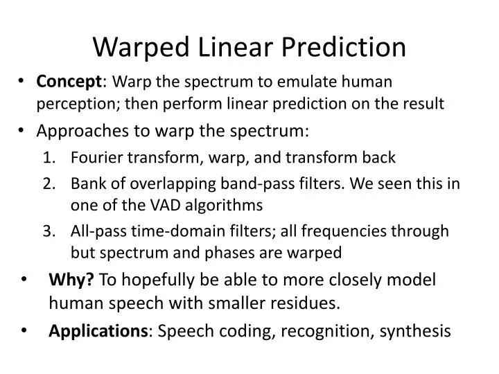
1. Warped Linear Prediction • Concept: Warp the spectrum to emulate human perception; then perform linear prediction on the result • Approaches to warp the spectrum: • Fourier transform, warp, and transform back • Bank of overlapping band-pass filters. We seen this in one of the VAD algorithms • All-pass time-domain filters; all frequencies through but spectrum and phases are warped • Why? To hopefully be able to more closely model human speech with smaller residues. • Applications: Speech coding, recognition, synthesis

2. All-pass filter • A pole of an all-phase filter lies inside the unit circle and the matching zero is outside. • The magnitudes of the matching poles and zeros cancel along the unit circle • They lie on the same radius line, so the polar coordinate angle is the same. • First order all pass filter transfer function: H(z) = B(z)/A(z) = (z-1 – p0*)/ (1-p0z-1) = (z-1- s e-jφ)/ (1-s ejφz-1) = (z-1- λ)/(1 - λz-1) • Example: if p0 = ½ + ½i, then the zero is at 1/p0* = 1/(½ - ½ i) = ( ½ + ½ i)/(1/2) = 1 + i • Higher order all pass filter s p0* r p0 Φ Note: p0* = conjugate of p an + an-1z-1 + an-2 z-2 + … + a1 z-n+1 + z-n H(z) = 1 + a1z-1 + a2 z-2 + … + an-1z-n+1 + anz-n

3. All pass Filter Visualization

4. All-pass Filter Phase Response • Real coefficients • λ, controls the location of the pole (p) and the zero (1/p). • No phase shift at frequencies 0, π, 2π; only a signal delay • Complex coefficients • Similar phase responses • Coefficients alter diagonal crossing frequency: fxfx = fs/2π arccos(λ) where fs is the sampling rate • Phase response: w+2arctan(λsin(w)/(1- λcos(w)) 2π λ= 0.8 Note: The cross over point is where there is no frequency warping, only a delay π 2π

5. Frequency Warping • All pass filter: magnitude remains constant, but the phase and frequency warped • Group delay • Definition: change of phase with respect to change of frequency • Interpretation: Different frequencies pass through a filter at different speeds. Therefore, a frequency warping operation occurs. • Formula: Where w is angle of original frequency, w’ is the angle of the warped frequency, λ is the all-pass coefficient (1- λ2)sin(w)(1- λ2) cos(w) - 2λ w’ = arctan

6. Illustration

7. Application to LPC • Warping to the match hearing auditory system • λ = 1.0674(2/π arctan(0.06583 fs/100) ½ -0.1916 • Significant at higher sampling rates: > 8k hz • CELP coding: • Degradation Mean Opinion Score (DMOS): 0.3 < λ < 0.4 • Best Bark Scale match: λ = 0.57 • Modified LPC: x’n = d * f; yn ≈ ∑k=1,N ak x’n • Convolute the frame, f, with all-pass filter, d • Apply linear prediction to warped frequency signal

8. Evaluation • Extra processing is minimal • The LPC estimate is more accurate than when warping is not used • For coding operations • Save one bit per sample at 48 kHz and 32 kHz • Save 0.6 bits per sample at 16kHz • Save 0.3 bits per sample at 8kHz • Less peaky residue spectrum than standard methods • Insignificant improvement for more than 30 LPC coefficients Matlab Toolbox: http://www.acoustics.hut.fi/software/warp

9. Inverse LPC Filter • Transfer function: Yz = Hz Xz • Xz is the original signal • Hz is the LPC filter ( G / (1-∑i=1,P ai z-i) • Yz is the filtered signal (residue) • Inverse filter: Yz / Hz = Xz • Yz is the filtered output • Hz is the LPC filter • Xz is the restored signal • Convolute the filtered signal with 1/Hz to restore the original signal from the residue

10. Click Detection using WLP • Definition: A click is a short localized discontinuity typically less than 1ms, which corrupts a signal • Clicked Detection with both Warped and Standard linear prediction • LPC: yk = ∑n=1,P an xk-n + rk + ck • rk is the residue and ck is the energy introduced by clicks • Looking for spikes (ck), can find click points • The warped linear prediction coefficient: λ • A value of 0.0 reverts to standard linear prediction • Positive values increase higher frequency resolution • Negative values increase lower frequency resolution

11. Click Detection Algorithm • Compute the standard deviation (σ) of the audio signal LPC residue (ex: the amount of residue that we expect to remain) • FOR each frame • Perform the Linear prediction with various λ values • Consider a click present in the frame when K σ > threshold, where K is an empirically set gain factor. • Approach 1 • Throw away frames determined to contain clicks • Disadvantage: some distortion is present • Approach 2 • Use interpolation to smooth the residue signal of clicks • Restore signal: Convolute the inverse LPC filter with the residue

12. Does WLP have an affect? • Prediction Gain (improvement in signal to noise ratio) • Divide clean signal energy by residue energy • Note: The residue is computed applying WLP to the noisy signal • The higher the result, the better the detection • Gp = 10 log (∑n=1,N |xn|2 / ∑n=1,n |rn|2) • Experiment • 44 kHz sample rate, 215 frames of 1024 samples, musical signal corrupted with known click points, λ values varied between -0.8 and +0.8 • Result: choice of λ affects the ratio between clean signal and residue with clicks

13. Experiment • Approach 1: Throw away click frames • Approach 2: Interpolate click frames • Results: • Both LPC and WLP can detect clicks • WLP with warping coefficient -0.7 reduces false detects • LPC and WLP miss approximately the same number of clicks