Download
1 / 52
520 likes | 530 Views
Comparing Populations. Proportions and means. The sampling distribution of differences of Normal Random Variables. If X and Y denote two independent normal random variables, then : D = X – Y is normal with. Comparing proportions. Situation We have two populations (1 and 2)

E N D
Comparing Populations Proportions and means
The sampling distribution of differences of Normal Random Variables If X and Y denote twoindependent normal random variables, then : D = X –Y is normal with
Comparing proportions Situation • We have two populations (1 and 2) • Let p1 denote the probability (proportion) of “success” in population 1. • Let p2 denote the probability (proportion) of “success” in population 2. • Objective is to compare the two population proportions
Consider the statistic: This statistic has a normal distribution
Consider the statistic: This statistic has a normal distribution with
Thus Has a standard normal distribution
We want to test either: or or
has a standard normal distribution. where is an estimate of the common value of p1 and p2.
Thus for comparing two binomial probabilities p1 and p2 The test statistic where
Example • In a national study to determine if there was an increase in mortality due to pipe smoking, a random sample of n1 = 1067 male nonsmoking pensioners were observed for a five-year period. • In addition a sample of n2 = 402 male pensioners who had smoked a pipe for more than six years were observed for the same five-year period. • At the end of the five-year period, x1 = 117 of the nonsmoking pensioners had died while x2 = 54 of the pipe-smoking pensioners had died. • Is there a the mortality rate for pipe smokers higher than that for non-smokers
We want to test: The test statistic:
We reject H0 if: Not true hence we accept H0. Conclusion: There is not a significant (a= 0.05) increase in the mortality rate due to pipe-smoking
Estimating a difference proportions using confidence intervals Situation • We have two populations (1 and 2) • Let p1 denote the probability (proportion) of “success” in population 1. • Let p2 denote the probability (proportion) of “success” in population 2. • Objective is to estimate the difference in the two population proportions d = p1 – p2.
Example • Estimating the increase in the mortality rate for pipe smokers higher over that for non-smokers d = p2 – p1
Comparing Means Situation • We have two normal populations (1 and 2) • Let m1and s1 denote the mean and standard deviation of population 1. • Let m2and s2 denote the mean and standard deviation of population 1. • Let x1, x2, x3 , … , xn denote a sample from a normal population 1. • Let y1, y2, y3 , … , ym denote a sample from a normal population 2. • Objective is to compare the two population means
or or We want to test either:
If: • will have a standard Normal distribution • This will also be true for the approximation (obtained by replacing s1 by sx and s2 by sy) if the sample sizes n and m are large (greater than 30)
Example • A study was interested in determining if an exercise program had some effect on reduction of Blood Pressure in subjects with abnormally high blood pressure. • For this purpose a sample of n = 500 patients with abnormally high blood pressure were required to adhere to the exercise regime. • A second sample m = 400 of patients with abnormally high blood pressure were not required to adhere to the exercise regime. • After a period of one year the reduction in blood pressure was measured for each patient in the study.
vs We want to test: The exercise group did not have a higher average reduction in blood pressure The exercise group did have a higher average reduction in blood pressure
We reject H0 if: True hence we reject H0. Conclusion: There is a significant (a= 0.05) effect due to the exercise regime on the reduction in Blood pressure
Estimating a difference means using confidence intervals Situation • We have two populations (1 and 2) • Let m1 denote the mean of population 1. • Let m2 denote the mean of population 2. • Objective is to estimate the difference in the two population proportions d = m1 – m2.
Example • Estimating the increase in the average reduction in Blood pressure due to the excercize regime d = m1 – m2
Comparing Means – small samples Situation • We have two normal populations (1 and 2) • Let m1and s1 denote the mean and standard deviation of population 1. • Let m2and s2 denote the mean and standard deviation of population 1. • Let x1, x2, x3 , … , xn denote a sample from a normal population 1. • Let y1, y2, y3 , … , ym denote a sample from a normal population 2. • Objective is to compare the two population means
We want to test either: or or
If the sample sizes (m and n) are large the statistic will have approximately a standard normal distribution This will not be the case if sample sizes (m and n) are small
The t test – for comparing means – small samples (equal variances) Situation • We have two normal populations (1 and 2) • Let m1and s denote the mean and standard deviation of population 1. • Let m2and s denote the mean and standard deviation of population 1. • Note: we assume that the standard deviation for each population is the same. s1 = s2 = s
The pooled estimate of s. Note: both sxand syare estimators of s. These can be combined to form a single estimator of s, sPooled.
The test statistic: If m1 = m2 this statistic has a t distribution with n + m –2 degrees of freedom
are critical points under the t distribution with degrees of freedom n + m –2.
Example • A study was interested in determining if administration of a drug reduces cancerous tumor size. • For this purpose n +m = 9 test animals are implanted with a cancerous tumor. • n = 3 are selected at random and administered the drug. • The remaining m = 6 are left untreated. • Final tumour sizes are measured at the end of the test period
We want to test: The treated group did not have a lower average final tumour size. vs The exercise group did have a lower average final tumour size.
We reject H0 if: with d.f. = n + m – 2 = 7 Hence we accept H0. Conclusion: The drug treatment does not result in a significant (a= 0.05) smaller final tumour size,