Download
1 / 24
620 likes | 1.88k Views
Singular Value Decomposition(SVD). Bo & Shi. Definition of SVD. Formally, the singular value decomposition of an m*n real or complex matrix M is a factorization of the form

E N D
Singular Value Decomposition(SVD) Bo & Shi
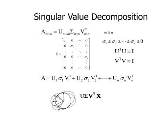
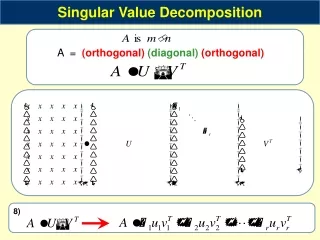
Definition of SVD • Formally, the singular value decomposition of an m*n real or complex matrix M is a factorization of the form • where U is an m*m real or complex unitary matrix, Σ is an m*n rectangular diagonal matrix with nonnegative real numbers on the diagonal, and V* (the conjugate transpose of V) is an n×n real or complex unitary matrix. The diagonal entries Σi,i of Σ are known as the singular values of M. The m columns of U and the n columns of V are called the left-singular vectors and right-singular vectors of M
Geometrical interpretation of SVD • for every linear map T:Kn → Km one can find orthonormal bases of Kn and Km such that T maps the i-th basis vector of Kn to a non-negative multiple of the i-th basis vector of Km, and sends the left-over basis vectors to zero. With respect to these bases, the map T is therefore represented by a diagonal matrix with non-negative real diagonal entries.
Geometrical interpretation of SVD • The SVD decomposes M into three simple transformations: a rotation V*, a scaling Σ along the rotated coordinate axes and a second rotation U.
Range, null-space, rank • Range • The range of A is the set of all vectors v for which the equation Ax = v has a solution. • Null-space • The null-space of A is the set of all the solutions to the equation Av = 0. • Rank • The rank of A is equal to its number of linearly independent columns, and also to its number of linearly independent rows.
SVD of a Square Matrix • If A is square matrix, then U,Σ and V are also square Matrix.
Condition number • the ratio of the largest(in magnitude) of the wj ’s to the smallest of the wj ’s. • (1) infinite: martrix is singular • (2)ill-conditoned : condition number is too large, that is, if its reciprocal approaches the machine’s floating-point precision
Three cases • 1. b=0. • 2. vector b on the right-hand side is not zero, and b lies in the range of A or not. • 3. b is not in the range of the singular matrix A.
First case • b=0 • It is solved immediately by SVD. • The solution is any linear combination of the columns returned by the nullspace method above.
Second case • Vector b on the right-hand side is not zero, and b lies in the range of A or not. • Specially, when =0. • This will be the solution vector of smallest length; the columns of V that are in the nullspace complete the specification of the solution set.
Third case • b is not in the range of the singular matrix A. • The number r is called the residual of the solution.
SVD for Fewer Equations than Unknowns • If we have fewer linear equations M than unknowns N, then we are not expecting a unique solution. Usually there will be an N*M dimensional family of solutions (which is the nullity, absent any other degeneracies), but the number could be larger. If we want to find this whole solution space, then SVD can readily do the job: Use solve to get one (the shortest) solution, then use nullspace to get a set of basis vectors for the nullspace. Our solutions are the former plus any linear combination of the latter.
Constructing an Orthonormal Basis • Construct an orthonormal basis for subspace by SVD: • Form an M*N matrix A whose N columns are our vectors. Construct an SVD object from the matrix. The columns of the matrix U are our desired orthonormal basis vectors.
Approximation of Matrices • The equation A=UWV can be rewritten to express any matrix as a sum of outer products of columns of U and rows of , with the “weighting factors” being the singular values
Advantage • If we ever encounter a situation where most of the singular values of a matrix A are very small, then A will be well-approximated by only a few terms in the sum. This means that we have to store only a few columns of U and V (the same k ones) and we will be able to recover, with good accuracy, the whole matrix.
Advantage • It is very efficient to multiply such an approximated matrix by a vector x: We just dot x with each of the stored columns of V, multiply the resulting scalar by the corresponding , and accumulate that multiple of the corresponding column of U. If our matrix is approximated by a small number K of singular values, then this computation of A·x takes only about K(M+N) multiplications, instead of MN for the full matrix.
Thank you • Reference • Numerical Recipes • Wikipedia about Singular Value Decomposition • Fundamentals of Computer Graphics