Download
1 / 37
370 likes | 510 Views
Soft X-Ray pulse length measurement. Alberto Lutman Jacek Krzywinski Juhao Wu Zhirong Huang Marc Messerschmidt …. 17.February.2011. Soft X-Ray Pulse length Determination. Electron Beam. Spectrometer. SASE FEL Amplifier. t. T. Goal: recover T from the spectra

E N D
Soft X-Ray pulse length measurement Alberto Lutman Jacek Krzywinski Juhao Wu Zhirong Huang Marc Messerschmidt … 17.February.2011
Soft X-Ray Pulse length Determination Electron Beam Spectrometer SASE FEL Amplifier t T Goal: recover T from the spectra (correlation technique proposed by Jacek K.)
Electron Beam Current profile tk is a random variable having probability density f(t) Current Fourier Transform t FEL transfer function in Exponential growth The spectrometer transfer function For Saturation, we run numerical simulations
Correlation of the radiation intensity at the exit of the spectrometer Frequencies that we correlate Single shot correlation, to be: averaged on many shots normalized Single shot spectrum
Calculation of the G2 function for different profiles To find an analytical expression for G2 we need just to plug in the f(t) function
Gaussian Electrons Profile * * G2 bunch profile ° ° # # M: “number of modes” With our spectrometer resolution, the rms of the bell shape is due to the spectrometer bandwidth
Flat top vs Gaussian G2 We cannot distinguish between: - Gaussian profile with rms length - Flat Top profile with full length
Some adressed Issues Statistical Gain Scales the measured function by Central Frequency Jitter
Numerical Simulations 1) Verified that relations hold well enough in saturation 2) Recover bunch length and spectrometer bandwith Bunch Length = 10 mm
A Matalab GUI to process the data Select a Subset of the collected spectra Plot spectra and Shot-to-shot recorded quantities Datasets Shot by shot quantities Calculate G2 Function Re-align Spectra Show Bunch Length Result
Bunch Length vs # of Undulators (2 November 2010 Data) FWHM Gaussian fs 13 16 19 25 22 28 Undulators
Spectrometer relative bandwidth (2 November 2010 Data) Spectrometer Relative bandwidth 13 16 19 22 25 28 Undulators
Bunch Length vs different peak current (26 January 2011 Data) FWHM Gaussian fs Peak current kA
Next Steps Include cases with non monoenergetic electron bunch - Two gaussian with different energies case - Including a linear energy chirp Analyze in detail data collected January 26 2011 Finish to write the paper Adapt the matlab GUI to be used in Control Room
Different pulses have different Gain Electron arrivals density probability T as a random variable with probability density p(t) Gain is function of T (e.g. smaller T, gives higher peak current and higher gain)
Statistical gain and FEL gain depending on profile length We are using indeed a different average profile The correlation function is affected by the statistical gain In case the gain is independent of T, the relation between G2 with and without the gain is the following:
Statistical gain and FEL gain depending on profile length We can observe that And get rid of this effect Using the offset of G2 normalizing shot by shot each spectrum with its energy Both approaches are not easy to apply when analyzing the real noisy spectral data
Gaussian Electrons Profile GASSIAN WITH SIGMA T
Statistical Gain Considering the model of incoherent radiation, the intensity at a certain frequency can be written We let the charge C fluctuate, and correlate intensities at two different frequencies w’ and w’’ with
Spectra Central Frequency jitter Considering the model of incoherent radiation, the intensity at a certain frequency can be written We let the charge C fluctuate, and correlate intensities at two different frequencies w’ and w’’ with
Different pulses have different Gain The G2 function is multiplied by
We can observe that for large To get rid of the multiplicative effect we can: Use the offset of G2s normalize shot by shot each spectrum with its integral Both approaches are not easy to apply when analyzing the real noisy spectral data
Numerical Simulations Flat top electrons profile Full Length = 10 um Radiation Wavelength = 1.5 A Rho = 4.5 x 10⁻⁴ Gain Length = 2.98 m Undulator Length = 100 m Number of Shots = 2000 Slippage Length = 0.5 um Analytical theory has been dereived in the linear regime. Simulation have been carried to determine if the theory is still applicable in saturation. Simulations have been also done for Gaussian electrons profile
Power vs Undulator Distance Gaussian electrons profile Flat top electrons profile
Flat top electrons profile Agreement: Z=30m Linear regime Z=60m saturation Z=100m Deep saturation
Flat top electrons profile 2 Agreement: Z=30m Linear regime 2 2 Z=60m saturation Z=100m Deep saturation
G2 function Flat top electrons profile
Simulations with Peak Current Jitter 30 m 60 m
Shot by Shot quantities For each shot, beside the spectra, other quantities have been recorded: x-ray pulse energy Electron bunch charge Electron bunch energy X and Y position X and Y angle Peak current
Filtering the datasets Theory assumes that different shots differ only by the arrival time of the electrons. This is not the case for the real data. We use the data collected to filter and keep only a subset of the spectra Filter: - bunch charge - bunch energy - peak current
Correlation between Energy and First moment The Gui allows to: show each spectrum profile plot recorded quantities Spectra first moment Electron bunch energy
Spectra Realignment We can realign the spectra, using the strong linear correlation between electron bunch energy and first moment We can either: Both approaches lead to the same bunch length result
Evaluation of the correlation function We calculate the correlation function. Interface leaves some freedom to: - Deal with backgroud noise issue - Deal with gain issue Bunch length is calculated with flat top and gaussian models
Results from data collected November 2nd, 2010 Only 6 sets of data collected with: 200 lines/mm monochromator 3 kA peak current Different number of undulators Can be used to calculate the bunch length. Other sets have: • Too low spectrometer resolution • Too low signal to noise ratio