Download
1 / 53
530 likes | 621 Views
Database and Knowledge Discovery : from Market Basket Data to Web PageRank. Jianlin Feng School of Software SUN YAT-SEN UNIVERSITY. What is a Database ?. A Database: A very large , integrated collection of data. Models a real-world “enterprise” Entities e.g., students, courses

E N D
Database and Knowledge Discovery:from Market Basket Data to Web PageRank Jianlin Feng School of Software SUN YAT-SEN UNIVERSITY
What is a Database ? • A Database: • A very large, integrated collection of data. • Models a real-world “enterprise” • Entities • e.g., students, courses • Relationships • e.g., Zhang San is taking the Database System course.
What is a Database Management System? • A Database Management System (DBMS) is: • A software system designed to store, manage, and facilitate query to databases. • Popular DBMS • Oracle • IBM DB2 • Microsoft SQL Server • Database System = Databases + DBMS
DBMS makes a big industry • The world's largest software companies by Forbes Global 2000 (http://www.forbes.com/lists/2009/18/global-09_The-Global-2000_IndName_17.html) • IBM • Microsoft • Oracle • Google • Softbank • SAP • Accenture • Computer Sciences Corporation • Yahoo! • Cap Gemini
Typical Applications Supported by Database Systems • Online Transaction Processing (OLTP) • Recording sales data in supermarkets • Booking flight tickets • Electronic banking • Online analytical processing (OLAP) and Data Warehousing • Business reporting for sales data • Customer Relationship Management (CRM)
Is the WWW a DBMS? • The Web = Surface Web + Deep Web • Surface Web: simply the HTML pages • Accessed by “search”: • Pose keywords in search box. • Deep Web: content hidden behind HTML forms Accessed by “query” • Fill in query forms.
“Search” vs. “Query” • Search is structure-free. • The keywords “database systems” can appear in anyplace in a HTML pages. • Query is structure-aware. • Say, we restruct that the keywords “database systems” can only appear in the “TITLE” field. • i.e., we assume there is an underlying STRUCTURE (of a book).
What is a “STUCTURE”? • Referring to the C programming language struct BOOK { char TITLE [256]; char AUTHOR [256]; float PRICE; int YEAR; } • In this course, we study database management systems that focus on processing structured data.
An Anecdote about “Search”:Google’s Founders are from Database Group of Stanford.
A Historical Perspective (1) • Relational Data Model, by Edgar Codd, 1970. • Codd, E.F. (1970). "A Relational Model of Data for Large Shared Data Banks". Communications of the ACM13 (6): 377–387. • Turing Award, 1981. • System R, by IBM, started in 1974 • Structured Query Language (SQL) • INGRES, by Berkeley, started in 1974 • POSTGRES, Mariposa, C-Store
A Historical Perspective (2) • Database Transaction Processing, mainly by Jim Gray. • J Gray, A Reuter. Transaction processing: concepts and techniques. 1993. • Turing Award, 1998. • Object-Relational DBMS, 1990s. • Stonebraker, Michael with Moore, Dorothy. Object-Relational DBMSs: The Next Great Wave. 1996. • Postgres (UC Berkeley), PostgreSQL. • IBM's DB2, Oracle database, and Microsoft SQL Server
Describing Data: Data Models • A data modelis a collection of concepts for describing data. • Aschemais a description of a particular collection of data, using a given data model. • The relational data model is the most widely used model today. • Main concept: relation, basically a table with rows and columns. • Every relation has a schema, which describes the columns, or fields (their names, types, constraints, etc.).
Schema in Relation Data Model A relation schema is a TEMPLATE of the corresponding relation. Definition of the Students Schema Students (sid: string, name: string, login: string, age: integer, gpa: real) Table 1. An Instance of the Students Relation
Queries in a Relational DBMS • Specified in a Non-Procedural way • Users only specify what data they need; • A DBMS takes care to evaluate queries as efficiently as possible. • a Non-Procedural Query Language: • SQL: Structured Query Language • Basic form of a SQL query: SELECT target-list FROMrelation-list WHERE qualification
A Simple SQL Example • At an airport, a gate agent clicks on a form to request the passenger list for a flight. SELECT name FROM Passenger Where flight = 510275 Passenger(pid: string, name: string, flight: integer)
Concurrent execution of user programs • Why? • Utilize CPU while waiting for disk I/O • (database programs make heavy use of disk) • Avoid short programs waiting behind long ones • e.g. ATM withdrawal while bank manager sums balance across all accounts courtesy of Joe Hellerstein
Concurrent execution • Interleaving actions of different user programs can lead to inconsistency: Example: • Bill transfers $100 from savings to checking Savings –= 100; Checking += 100 • Meanwhile, Bill’s wife requests account info. Bad interleaving: • Savings –= 100 • Print balances • Checking += 100 • Printout is missing $100 ! courtesy of Joe Hellerstein
Concurrency Control • DBMS ensures such problems don’t arise. • Users can pretend they are using a single-user system.
The Market-Basket Model • A large set of items, e.g., things sold in a supermarket. • A large set of baskets, each of which is a small set of the items, e.g., the things one customer buys on one day.
Support • Simplest question: find sets of items that appear “frequently” in the baskets. • Support for itemset I = the number of baskets containing all items in I. • Sometimes given as a percentage. • Given a supportthresholds, sets of items that appear in at least s baskets are called frequent itemsets.
, {b,c} , {c,j}. {m,b} Example: Frequent Itemsets • Items={milk, coke, pepsi, beer, juice}. • Support = 3 baskets. B1 = {m, c, b} B2 = {m, p, j} B3 = {m, b} B4 = {c, j} B5 = {m, p, b} B6 = {m, c, b, j} B7 = {c, b, j} B8 = {b, c} • Frequent itemsets: {m}, {c}, {b}, {j},
Applications – (1) • Items = products; baskets = sets of products someone bought in one trip to the store. • Exampleapplication: given that many people buy beer and diapers together: • Run a sale on diapers; raise price of beer. • Only useful if many buy diapers & beer.
Applications – (2) • Baskets = Web pages; items = words. • Unusual words appearing together in a large number of documents, e.g., “Brad” and “Angelina,” may indicate an interesting relationship.
Association Rules • If-then rules about the contents of baskets. • {i1, i2,…,ik} →jmeans: “if a basket contains all of i1,…,ik then it is likely to contain j.” • Confidence of this association rule is the probability of j given i1,…,ik.
Example: Confidence B1 = {m, c, b} B2 = {m, p, j} B3 = {m, b} B4 = {c, j} B5 = {m, p, b} B6 = {m, c, b, j} B7 = {c, b, j} B8 = {b, c} • An association rule: {m, b} →c. • Confidence = 2/4 = 50%. + _ _ +
Finding Association Rules • Question: “find all association rules with support ≥s and confidence ≥c .” • Note: “support” of an association rule is the support of the set of items on the left. • Hard part: finding the frequent itemsets. • Note: if {i1, i2,…,ik} →j has high support and confidence, then both {i1, i2,…,ik} and {i1, i2,…,ik ,j} will be “frequent.”
A-Priori Algorithm – (1) • A two-pass approach called a-priori limits the need for main memory. • Key idea: monotonicity : if a set of items appears at least s times, so does every subset. • Contrapositive for pairs: if item i does not appear in s baskets, then no pair including i can appear in s baskets.
A-Priori Algorithm – (2) • Pass 1: Read baskets and count in main memory the occurrences of each item. • Requires only memory proportional to #items. • Items that appear at least s times are the frequent items.
A-Priori Algorithm – (3) • Pass 2: Read baskets again and count in main memory only those pairs both of which were found in Pass 1 to be frequent. • Requires memory proportional to square of frequent items only (for counts), plus a list of the frequent items (so you know what must be counted).
Picture of A-Priori Item counts Frequent items Counts of pairs of frequent items Pass 1 Pass 2
Page Rank: Ranking web pages • Web pages are not equally “important” • www.joe-schmoe.com v www.stanford.edu • Inlinks as votes • www.stanford.edu has 23,400 inlinks • www.joe-schmoe.com has 1 inlink • Are all inlinks equal? • Recursive question!
Simple recursive formulation • Each link’s vote is proportional to the importance of its source page • If page P with importance x has n outlinks, each link gets x/n votes • Page P’s own importance is the sum of the votes on its inlinks
Yahoo Amazon M’soft Simple “flow” model The web in 1839 y = y /2 + a /2 a = y /2 + m m = a /2 y/2 y a/2 y/2 m a/2 m a
Solving the flow equations • 3 equations, 3 unknowns, no constants • No unique solution • All solutions equivalent modulo scale factor • Additional constraint forces uniqueness • y+a+m = 1 • y = 2/5, a = 2/5, m = 1/5 • Gaussian elimination method works for small examples, but we need a better method for large graphs
Matrix formulation • Matrix M has one row and one column for each web page • Suppose page j has n outlinks • If j i, then Mij=1/n • Else Mij=0 • M is a columnstochastic matrix • Columns sum to 1 • Suppose r is a vector with one entry per web page • ri is the importance score of page i • Call it the rank vector • |r| = 1
j i i = 1/3 M r Example Suppose page j links to 3 pages, including i r
Eigenvector formulation • The flow equations can be written r = Mr • So the rank vector is an eigenvector of the stochastic web matrix • In fact, its first or principal eigenvector, with corresponding eigenvalue 1
Yahoo r = Mr Amazon M’soft y 1/2 1/2 0 y a = 1/2 0 1 a m 0 1/2 0 m Example y a m y 1/2 1/2 0 a 1/2 0 1 m 0 1/2 0 y = y /2 + a /2 a = y /2 + m m = a /2
Power Iteration method • Simple iterative scheme (aka relaxation) • Suppose there are N web pages • Initialize: r0 = [1/N,….,1/N]T • Iterate: rk+1 = Mrk • Stop when |rk+1 - rk|1 < • |x|1 = 1≤i≤N|xi| is the L1 norm • Can use any other vector norm e.g., Euclidean
Yahoo Amazon M’soft Power Iteration Example y a m y 1/2 1/2 0 a 1/2 0 1 m 0 1/2 0 y a = m 1/3 1/3 1/3 1/3 1/2 1/6 5/12 1/3 1/4 3/8 11/24 1/6 2/5 2/5 1/5 . . .
Random Walk Interpretation • Imagine a random web surfer • At any time t, surfer is on some page P • At time t+1, the surfer follows an outlink from P uniformly at random • Ends up on some page Q linked from P • Process repeats indefinitely • Let p(t) be a vector whose ith component is the probability that the surfer is at page i at time t • p(t) is a probability distribution on pages
The stationary distribution • Where is the surfer at time t+1? • Follows a link uniformly at random • p(t+1) = Mp(t) • Suppose the random walk reaches a state such that p(t+1) = Mp(t) = p(t) • Then p(t) is called a stationary distribution for the random walk • Our rank vector r satisfies r = Mr • So it is a stationary distribution for the random surfer
Existence and Uniqueness A central result from the theory of random walks (aka Markov processes): For graphs that satisfy certain conditions, the stationary distribution is unique and eventually will be reached no matter what the initial probability distribution at time t = 0.
Spider traps • A group of pages is a spider trap if there are no links from within the group to outside the group • Random surfer gets trapped • Spider traps violate the conditions needed for the random walk theorem
Microsoft becomes a spider trap Yahoo y a m y 1/2 1/2 0 a 1/2 0 0 m 0 1/2 1 Amazon M’soft y a = m 1 1 1 1 1/2 3/2 3/4 1/2 7/4 5/8 3/8 2 0 0 3 . . .
Random teleports • The Google solution for spider traps • At each time step, the random surfer has two options: • With probability , follow a link at random • With probability 1-, jump to some page uniformly at random • Common values for are in the range 0.8 to 0.9 • Surfer will teleport out of spider trap within a few time steps
y y y 1/3 1/3 1/3 y 1/2 a 1/2 m 0 1/2 1/2 0 + 0.2* 0.8* Random teleports ( = 0.8) 0.2*1/3 1/2 Yahoo 0.8*1/2 1/2 0.2*1/3 0.8*1/2 0.2*1/3 1/2 1/2 0 1/2 0 0 0 1/2 1 1/3 1/3 1/3 1/3 1/3 1/3 1/3 1/3 1/3 + 0.2 Amazon M’soft 0.8 y 7/15 7/15 1/15 a 7/15 1/15 1/15 m 1/15 7/15 13/15