Download
1 / 63
630 likes | 745 Views
Logic Synthesis in IC Design and Associated Tools The MIS Tool. Wang Jiang Chau Grupo de Projeto de Sistemas Eletrônicos e Software Aplicado Laboratório de Microeletrônica – LME Depto. Sistemas Eletrônicos Universidade de São Paulo. MIS: Multilevel Logic Optimizer.

E N D
Logic Synthesis in IC Design and Associated Tools The MIS Tool Wang Jiang Chau Grupo de Projeto de Sistemas Eletrônicos e Software Aplicado Laboratório de Microeletrônica – LME Depto. Sistemas Eletrônicos Universidade de São Paulo
MIS: Multilevel Logic Optimizer • Includes decomposition, minimization and technology mapping • Supports command-line and script interface • Aimed to static CMOS • Both local and global optimization • Based on kernel extraction and (algebraic and Boolean) division algorithms
MIS… • All previous definitions hold (support, literal, cofactor, etc.) • Alternate form to Sum-of-products (SOPs) • Factored form- recursive definition • A literal is a factored form • The sum of a factored form is also a factored form • The product of a factored form is also a factored form Objective: a minimal factored form (???)
Circuit Modeling • Logic network • Interconnection of logic functions. • Hybrid structural/behavioral model. • Bound (mapped) networks • Interconnection of logic gates. • Structural model. Example of Bound Network
Network Optimization • Two-level logic • Area and delay proportional to cover size. • Achieving minimum (or irredundant) covers corresponds to optimizing area and speed. • Achieving irredundant cover corresponds to maximizing testability. • Multiple-level logic • Minimal-area implementations do not correspond in general to minimum-delay implementations and vice versa. • Minimize area (power) estimate • subject to delay constraints. • Minimize maximum delay • subject to area (power) constraints. • Minimize power consumption. • subject to delay constraints. • Maximize testability.
Estimation • Area • Number of literals • Corresponds to number of polysilicon strips (transistors) • Number of functions/gates. • Delay • Number of stages (unit delay per stage). • Refined gate delay models (relating delay to function complexity and fanout). • Sensitizable paths (detection of false paths). • Wiring delays estimated using statistical models.
Problem Analysis • Multiple-level optimization is hard. • Exact methods • Exponential complexity. • Impractical. • Approximate methods • Heuristic algorithms. • Rule-based methods. • Strategies for optimization • Improve circuit step by step based on circuit transformations. • Preserve network behavior. • Methods differ in • Types of transformations. • Selection and order of transformations.
Elimination • Eliminate one function from the network. • Perform variable substitution. • Example • s = r +b’; r = p+a’ s = p+a’+b’.
Decomposition • Break one function into smaller ones. • Introduce new vertices in the network. • Example • v = a’d+bd+c’d+ae’. j = a’+b+c’; v = jd+ae’
Factoring • Factoring is the process of deriving a factored form from a sum-of-products form of a function. • Factoring is like decomposition except that no additional nodes are created. • Example • F = abc+abd+a’b’c+a’b’d+ab’e+ab’f+a’be+a’bf (24 literals) • After factorization • F=(ab+a’b’)(c+d) + (ab’+a’b)(e+f) (12 literals)
Extraction - 1 • Find a common sub-expression of two (or more) expressions. • Extract sub-expression as new function. • Introduce new vertex in the network. • Example • p = ce+de; t = ac+ad+bc+bd+e; (13 literals) • p = (c+d)e; t = (c+d)(a+b)+e; (Factoring:8 literals) k = c+d; p = ke; t = ka+ kb +e; (Extraction:9 literals)
Simplification • Simplify a local function (using Espresso). • Example • u = q’c+qc’ +qc; u = q +c;
Substitution • Simplify a local function by using an additional input that was not previously in its support set. • Example • t = ka+kb+e. t = kq +e; because q = a+b.
Example: Sequence of Transformations Original Network (33 lit.) Transformed Network (20 lit.)
Optimization Approaches • Algorithmic approach • Define an algorithm for each transformation type. • Algorithm is an operator on the network. • Each operator has well-defined properties • Heuristic methods still used. • Weak optimality properties. • Sequence of operators • Defined by scripts. • Based on experience. • Rule-based approach (IBM Logic Synthesis System) • Rule-data base • Set of pattern pairs. • Pattern replacement driven by rules.
Elimination Algorithm - 1 • Set a threshold k (usually 0). • Examine all expressions (vertices) and compute their values. • Vertex value = n*l – n – l (l is number of literals; n is number of times vertex variable appears in network) • Eliminate an expression (vertex) if its value (i.e. the increase in literals) does not exceed the threshold.
Elimination Algorithm - 2 • Example • q = a + b • s = ce + de + a’ + b’ • t = ac + ad + bc + bd + e • u = q’c + qc’ + qc • v = a’d + bd + c’d + ae’ • Value of vertex q=n*l–n–l=3*2-3-2=1 • It will increase number of literals => not eliminated • Assume u is simplified to u=c+q • Value of vertex q=n*l–n–l=1*2-1-2=-1 • It will decrease the number of literals by 1 => eliminated
MIS/SIS Rugged Script Sweep eliminates single-input Vertices and those with a constant function. • sweep; eliminate -1 • simplify -m nocomp • eliminate -1 • sweep; eliminate 5 • simplify -m nocomp • resub -a • fx • resub -a; sweep • eliminate -1; sweep • full-simplify -m nocomp resub–a performs algebraic substitution of all vertex pairs fx extracts double-cube and single-cube expression.
Boolean and Algebraic Methods - 1 • Boolean methods • Exploit Boolean properties of logic functions. • Use don't care conditions induced by interconnections. • Complex at times. • Algebraic methods • View functions as polynomials. • Exploit properties of polynomial algebra. • Simpler, faster but weaker.
Boolean and Algebraic Methods - 2 • Boolean substitution • h = a+bcd+e; q = a+cd h = a+bq +e • Because a+bq+e = a+b(a+cd)+e = a+bcd+e; • Relies on Boolean property b+1=1 • Algebraic substitution • t = ka+kb+e; q=a+b t = kq +e • Because k(a+b) = ka+kb; holds regardless of any assumption of Boolean algebra.
The Algebraic Model - 1 • Represents local Boolean functions by algebraic expressions • Multilinear polynomial (i.e. multi-variable with degree 1) over set of variables with unit coefficients. • Algebraic transformations neglect specific features of Boolean algebra • Only one distributive law applies • a . (b+c) = ab+ac • a + (b . c) (a+b).(a+c) • Complements are not defined • Cannot apply some properties like absorption, idempotence, involution and Demorgan’s, a+a’=1 and a.a’=0 • Symmetric distribution laws. • Don't care sets are not used.
The Algebraic Model - 2 • Algebraic expressions obtained by • Modeling functions in sum of products form. • Make them minimal with respect to single-cube containment. • Algebraic operations restricted to expressions with disjoint support • Preserve correspondence of result with sum-of-product forms minimal w.r.t single-cube containment. • Example • (a+b)(c+d)=ac+ad+bc+bd; minimal w.r.t SCC. • (a+b)(a+c)= aa+ac+ab+bc; non-minimal. • (a+b)(a’+c)=aa’+ac+a’b+bc; non-minimal.
Divisor - 1 • Given two algebraic expressions fdividend and fdivisor , • we say that fdivisor is an Algebraic Divisor of fdividend , fquotient = fdividend/fdivisor when • fdividend = fdivisor . fquotient + fremainder • fdivisor . fquotient 0 • and the support of fdivisor and fquotient is disjoint. • we say that fdivisor is an Boolean Divisor of fdividend , fquotient = fdividend/fdivisor when • fdividend = fdivisor . fquotient + fremainder • fdivisor . fquotient 0
Divisor - 2 • Example • Let fdividend = ac+ad+bc+bd+e and fdivisor = a+b • Then fquotient = c+d fremainder = e • because (a+b) (c+d)+e = fdividend • Therefore, a+b is a Bolean divisor • Since {a,b} {c,d} = , a+b is also an algebraic divisor • Let fi = a+bc and fj = a+b. • Let fk = a+c. Then, fi = fj . fk = (a+b)(a+c) = fi • Since{a,b} {a,c} , a+b is only a Boolean divisor
Factor - 1 • An algebraic (Boolean) divisor is called an algebraic (Boolean) factor whenever the remainder is void. • a+b is a (Boolean and algebraic) factor of ac+ad+bc+bd • Lema: if g is an algebraic divisor (factor) of f, then, g is a Boolean divisor (factor) of f. • Property: for fdividend = fdivisor . fquotient + fremainder , if fdivisor is an algebraic divisor, then fquotient is unique If fdivisor is a Boolean divisor, then fquotient is non-unique
Division • The basic operation to be performed, given f an g, is f=g.h+r • There are two problems to be solved: Problem 1: how to get the “best” h ? problem of division Problem 2: how to get the “best” g ? problem of kernel extraction • Property: given f and g, the algebraic division is faster than the Boolean division
Algebraic Division Algorithm - 1 • Quotient Q and remainder R are sum of cubes (monomials). • Intersection is largest subset of common monomials.
Algebraic Division Algorithm - 2 • Example • fdividend = ac+ad+bc+bd+e; • fdivisor = a+b; • A = {ac, ad, bc, bd, e} and B = {a, b}. • i = 1 • CB1 = a, D = {ac, ad} and D1 = {c, d}. • Q = {c, d}. • i = 2 = n • CB2 = b, D = {bc, bd} and D2 = {c, d}. • Then Q = {c, d} {c, d} = {c, d}. • Result • Q = {c, d} and R = {e}. • fquotient = c+d and fremainder = e.
Algebraic Division Algorithm - 3 • Example • Let fdividend = axc+axd+bc+bxd+e; fdivisor = ax+b • i=1, CB1 = ax, D = {axc, axd} and D1 = {c, d}; Q={c, d} • i = 2 = n; CB2 = b, D = {bc, bxd} and D2 = {c, xd}. • Then Q = {c, d} {c, xd} = {c}. • fquotient = c and fremainder = axd+bxd+e. • Theorem: Given algebraic expressions fi and fj, then fi/fj is empty when • fj contains a variable not in fi. • fj contains a cube whose support is not contained in that of any cube of fi. • fj contains more cubes than fi. • The count of any variable in fj larger than in fi.
Kernels- 1 Definition: An expression composed of two or more cubes is cube-free if no cube divides the expression evenly (i.e. there is no literal that is common to all the cubes). ab + c is cube-free (no cube divides both ab and c) ab + ac is not cube-free (a divides both ab and ac) abd + acd is not cube-free (ad divides both abd and acd) abc is not cube-free (only one cubea cube-free expression must have more than one cube) Definition: The primary divisors of an expression F are the set of expressionsD(F) = {F/c | c is a cube}.
Kernels- 2 Definition: The kernels of an expression F are the set of expressionsK(F) = {G | G D(F) and G is cube-free}. In other words, the kernels of an expression F are the cube-free primary divisors of F. Definition: A cube c used to obtain the kernel K = F/c is called a co -kernels of F
Example Example: x = adf + aef + bdf + bef + cdf + cef + g= (a + b + c)(d + e)f + g kernelsco-kernels a+b+c df, ef d+e af, bf, cf (a+b+c)(d+e) f (a+b+c)(d+e)f+g 1
The Level of a Kernel Definition: A kernel is of level 0 (K0) if it contains no kernels except itself. A kernel is of level n (Kn) if it contains at least one kernel of level (n-1), but no kernels (except itself) of level n or greater • K0(F) K1(F) K2(F) ... Kn(F) K(F). • level-n kernels = Kn(F) \ Kn-1(F) • Kn(F) is the set of kernels of level k or less. Example:F = (a + b(c + d))(e + g) k1 = a + b(c + d) K1 K0 ==> level-1 k2 = c + d K0 k3 = e + g K0
Kernel Set Computation • Naive method • Divide function by elements in power set of its support set. • Weed out non cube-free quotients. • Smart way • Use recursion • Kernels of kernels are kernels of original expression. • Exploit commutativity of multiplication. • Kernels with co-kernels ab and ba are the same • A kernel has level 0 if it has no kernel except itself. • A kernel is of level n if it has • at least one kernel of level n-1 • no kernels of level n or greater except itself
Naive Method-Example • fx = ace+bce+de+g • Divide fx by a. Get ce. Not cube free. • Divide fx by b. Get ce. Not cube free. • Divide fx by c. Get ae+be. Not cube free. • Divide fx by ce. Get a+b. Cube free. Kernel! • Divide fx by d. Get e. Not cube free. • Divide fx by e. Get ac+bc+d. Cube free. Kernel! • Divide fx by g. Get 1. Not cube free. • Expression fx is a kernel of itself because cube free. • K(fx) = {(a+b); (ac+bc+d); (ace+bce+de+g)}.
Recursive Kernel Computation: Simple Algorithm Definition: Given a function (SOP cover) F and a cube x, Cube (F,x) = {ci | ciF and s.t. literal x also ci} • f is assumed to be cube-free and minimized • If not (cube-free), divide it by its largest cube factor
Recursive Kernel Computation Example- 1 • f = ace+bce+de+g • Literals a or b. No action required. • Literal c. Select cube ce: • Recursive call with argument (ace+bce+de+g)/ce =a+b; • No additional kernels. • Adds a+b to the kernel set at the last step. • Literal d. No action required. • Literal e. Select cube e: • Recursive call with argument ac+bc+d • Kernel a+b is rediscovered and added. • Adds ac + bc + d to the kernel set at the last step. • Literal g. No action required. • Adds ace+bce+de+g to the kernel set. • K = {(ace+bce+de+g); (a+b); (ac+bc+d); (a+b)}.
Recursive Kernel Computation Example- 2 • Y= adf + aef + bdf + bef + cdf + cef + g=(d+e)(a+b+c)f+g • Lexicographic order {a, b, c, d, e, f, g} adf + aef + bdf + bef + cdf + cef + g af df ef bf f cf a+b+c d+e d+e a+b+c d+e ad+ae+bd+be+cd+ce
Analysis • Some computation may be redundant • Example • Divide by a and then by b. • Divide by b and then by a. • Obtain duplicate kernels. • Improvement • Keep a pointer to literals used so far denoted by j. • J initially set to 1. • Avoids generation of co-kernels already calculated • Sup(f)={x1, x2, …xn} (arranged in lexicographic order) • f is assumed to be cube-free • If not divide it by its largest cube factor • Faster algorithm
New Recursive Kernel Computation Examples- 1 • f = ace+bce+de+g; sup(f)={a, b, c, d, e, g} • Literals a or b. No action required. • Literal c. Select cube ce: • Recursive call with arguments: (ace+bce+de+g)/ce =a+b; pointer j = 3+1=4. • Call considers variables {d, e, g}. No kernel. • Adds a+b to the kernel set at the last step. • Literal d. No action required. • Literal e. Select cube e: • Recursive call with arguments: ac+bc+d and pointer j = 5+1=6. • Call considers variable {g}. No kernel. • Adds ac+bc+d to the kernel set at the last step. • Literal g. No action required. • Adds ace+bce+de+g to the kernel set. • K = {(ace+bce+de+g); (ac+bc+d); (a+b)}. • Now:lets try´do it again after trading de by de’
New Recursive Kernel Computation Examples- 2 abcd + abce + adfg + aefg + adbe + acdef + beg (bc + fg)(d + e) + de(b + cf) c (a) a b (a) b g e c c d f d (a) e cd+g d+e ac+d+g d c d e e f d+e c+d b+ef b+df b+cf ce+g c+e a(d+e) c(d+e) + de= d(c+e) + ce = ...
Extraction • Search for common sub-expressions • Single-cube extraction: monomial. • Multiple-cube (kernel) extraction: polynomial • Search for appropriate divisors. • Cube-free expression • Cannot be factored by a cube. • Kernel of an expression • Cube-free quotient of the expression divided by a cube (called co-kernel). • Kernel set K(f) of an expression • Set of kernels.
Single-Cube Extraction - 1 • Form auxiliary function • Sum of all product terms of all functions. • Methods: • Find the kernels (and co-kernels) • Form matrix representation • A rectangle with at least two rows represents a common cube. • Rectangles with at least two columns may result in savings. • Best choice is a prime rectangle. • Use function ID for cubes • Cube intersection from different functions.
Single-Cube Extraction - 2 • Expressions • fx = ace+bce+de+g • fs = cde+b • Auxiliary function • faux = ace+bce+de+g + cde+b • Kernels (except single literals): (a+b+c)ce care must be taken • Matrix: • Prime rectangle: ({1, 2, 5}ce, {3, 5}de) • Extract cube ce.
Single-Cube Extraction Algorithm Extraction of an l-variable cube with multiplicity n saves (n l – n – l) literals
Multiple-Cube Extraction - 1 • We need a kernel/cube matrix. • Relabeling • Cubes by new variables. • Kernels by cubes. • Form auxiliary function • Sum of all kernels. • Methods: • Find the kernels (and co-kernels) • Extend cube intersection algorithm.
Method 1 • Relabeling • fp = ace+bce: ace x1; bce x2 • fp = x1.x2 • fq = ae+be+d: ae x3; be x4 ; d x5 • fq = x3.x4 .x5 • fr = ae+be+df: ae x3; be x4 ; de x6 • fr = x3.x4 .x6 • faux = x1.x2 + x3.x4 .x5 + x3.x4 .x6. • K(faux) = {(x5+x6)} • C(faux) = {(x3.x4)}. • Re-relabeling. • x3.x4 (ae+be) (not eit is not cube-free).