Download
1 / 43
430 likes | 570 Views
CS6670: Computer Vision. Noah Snavely. Lecture 15: Eigenfaces. Announcements. Wednesday’s class is cancelled My office hours moved to tomorrow (Tuesday) 1:30-3:00. Dimensionality reduction. The set of faces is a “subspace” of the set of images Suppose it is K dimensional

E N D
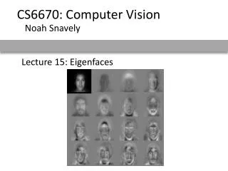
CS6670: Computer Vision Noah Snavely Lecture 15: Eigenfaces
Announcements • Wednesday’s class is cancelled • My office hours moved to tomorrow (Tuesday) 1:30-3:00
Dimensionality reduction • The set of faces is a “subspace” of the set of images • Suppose it is K dimensional • We can find the best subspace using PCA • This is like fitting a “hyper-plane” to the set of faces • spanned by vectors v1, v2, ..., vK • any face
Eigenfaces • PCA extracts the eigenvectors of A • Gives a set of vectors v1, v2, v3, ... • Each one of these vectors is a direction in face space • what do these look like?
Projecting onto the eigenfaces • The eigenfaces v1, ..., vK span the space of faces • A face is converted to eigenface coordinates by
Detection and recognition with eigenfaces • Algorithm • Process the image database (set of images with labels) • Run PCA—compute eigenfaces • Calculate the K coefficients for each image • Given a new image (to be recognized) x, calculate K coefficients • Detect if x is a face • If it is a face, who is it? • Find closest labeled face in database • nearest-neighbor in K-dimensional space
i = K NM Choosing the dimension K • How many eigenfaces to use? • Look at the decay of the eigenvalues • the eigenvalue tells you the amount of variance “in the direction” of that eigenface • ignore eigenfaces with low variance eigenvalues
Issues: metrics • What’s the best way to compare images? • need to define appropriate features • depends on goal of recognition task classification/detectionsimple features work well(Viola/Jones, etc.) exact matchingcomplex features work well(SIFT, MOPS, etc.)
Metrics • Lots more feature types that we haven’t mentioned • moments, statistics • metrics: Earth mover’s distance, ... • edges, curves • metrics: Hausdorff, shape context, ... • 3D: surfaces, spin images • metrics: chamfer (ICP) • ...
If you have a training set of images:AdaBoost, etc. Issues: feature selection If all you have is one image:non-maximum suppression, etc.
Issues: data modeling • Generative methods • model the “shape” of each class • histograms, PCA, mixtures of Gaussians • graphical models (HMM’s, belief networks, etc.) • ... • Discriminative methods • model boundaries between classes • perceptrons, neural networks • support vector machines (SVM’s)
Generative vs. Discriminative Generative Approachmodel individual classes, priors Discriminative Approachmodel posterior directly from Chris Bishop
Issues: dimensionality • What if your space isn’t flat? • PCA may not help Nonlinear methodsLLE, MDS, etc.
Issues: speed • Case study: Viola Jones face detector • Exploits two key strategies: • simple, super-efficient features • pruning (cascaded classifiers) • Next few slides adapted Grauman & Liebe’s tutorial • http://www.vision.ee.ethz.ch/~bleibe/teaching/tutorial-aaai08/ • Also see Paul Viola’s talk (video) • http://www.cs.washington.edu/education/courses/577/04sp/contents.html#DM
Feature extraction “Rectangular” filters • Feature output is difference between adjacent regions Value at (x,y) is sum of pixels above and to the left of (x,y) • Efficiently computable with integral image: any sum can be computed in constant time • Avoid scaling images scale features directly for same cost Integral image Viola & Jones, CVPR 2001 15 K. Grauman, B. Leibe K. Grauman, B. Leibe
Large library of filters • Considering all possible filter parameters: position, scale, and type: • 180,000+ possible features associated with each 24 x 24 window Use AdaBoost both to select the informative features and to form the classifier Viola & Jones, CVPR 2001 K. Grauman, B. Leibe
AdaBoost for feature+classifier selection Want to select the single rectangle feature and threshold that best separates positive (faces) and negative (non-faces) training examples, in terms of weighted error. Resulting weak classifier: For next round, reweight the examples according to errors, choose another filter/threshold combo. … Outputs of a possible rectangle feature on faces and non-faces. Viola & Jones, CVPR 2001 K. Grauman, B. Leibe
AdaBoost: Intuition Consider a 2-d feature space with positive and negative examples. Each weak classifier splits the training examples with at least 50% accuracy. Examples misclassified by a previous weak learner are given more emphasis at future rounds. Figure adapted from Freund and Schapire 18 K. Grauman, B. Leibe K. Grauman, B. Leibe
AdaBoost: Intuition 19 K. Grauman, B. Leibe K. Grauman, B. Leibe
AdaBoost: Intuition Final classifier is combination of the weak classifiers 20 K. Grauman, B. Leibe K. Grauman, B. Leibe
AdaBoost Algorithm Start with uniform weights on training examples {x1,…xn} For T rounds Evaluate weighted error for each feature, pick best. Re-weight the examples: Incorrectly classified -> more weight Correctly classified -> less weight Final classifier is combination of the weak ones, weighted according to error they had. Freund & Schapire 1995 K. Grauman, B. Leibe
Cascading classifiers for detection Fleuret & Geman, IJCV 2001 Rowley et al., PAMI 1998 Viola & Jones, CVPR 2001 For efficiency, apply less accurate but faster classifiers first to immediately discard windows that clearly appear to be negative; e.g., • Filter for promising regions with an initial inexpensive classifier • Build a chain of classifiers, choosing cheap ones with low false negative rates early in the chain 22 Figure from Viola & Jones CVPR 2001 K. Grauman, B. Leibe K. Grauman, B. Leibe
Viola-Jones Face Detector: Summary Train cascade of classifiers with AdaBoost Apply to each subwindow Faces New image Selected features, thresholds, and weights Non-faces Train with 5K positives, 350M negatives Real-time detector using 38 layer cascade 6061 features in final layer [Implementation available in OpenCV: http://www.intel.com/technology/computing/opencv/] 23 K. Grauman, B. Leibe
Viola-Jones Face Detector: Results First two features selected 24 K. Grauman, B. Leibe K. Grauman, B. Leibe
Viola-Jones Face Detector: Results K. Grauman, B. Leibe
Viola-Jones Face Detector: Results K. Grauman, B. Leibe
Viola-Jones Face Detector: Results K. Grauman, B. Leibe
Detecting profile faces? Detecting profile faces requires training separate detector with profile examples. K. Grauman, B. Leibe
Viola-Jones Face Detector: Results Paul Viola, ICCV tutorial K. Grauman, B. Leibe
Questions? • 3-minute break
Moving forward • Faces are pretty well-behaved • Mostly the same basic shape • Lie close to a subspace of the set of images • Not all objects are as nice
Bag of Words Models Adapted from slides by Rob Fergus
Object Bag of ‘words’
Bag of Words • Independent features • Histogram representation
1.Feature detectionand representation Compute descriptor e.g. SIFT [Lowe’99] Normalize patch Detect patches [Mikojaczyk and Schmid ’02] [Mata, Chum, Urban & Pajdla, ’02] [Sivic & Zisserman, ’03] Local interest operator or Regular grid Slide credit: Josef Sivic
… 1.Feature detectionand representation
… 2. Codewords dictionary formation 128-D SIFT space
… 2. Codewords dictionary formation Codewords + + + Vector quantization 128-D SIFT space Slide credit: Josef Sivic
Image patch examples of codewords Sivic et al. 2005
….. Image representation Histogram of features assigned to each cluster frequency codewords
Uses of BoW representation • Treat as feature vector for standard classifier • e.g k-nearest neighbors, support vector machine • Cluster BoW vectors over image collection • Discover visual themes