Download
1 / 42
420 likes | 595 Views
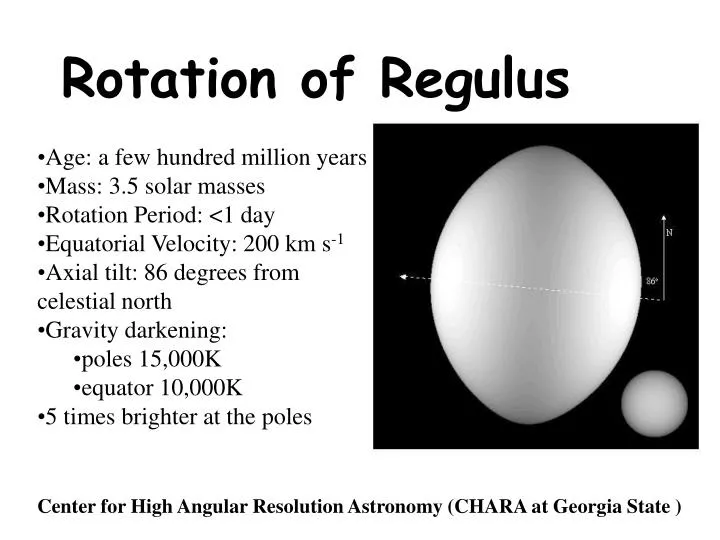
Rotation of Regulus. Age: a few hundred million years Mass: 3.5 solar masses Rotation Period: <1 day Equatorial Velocity: 200 km s -1 Axial tilt: 86 degrees from celestial north Gravity darkening: poles 15,000K equator 10,000K 5 times brighter at the poles.

E N D
Rotation of Regulus • Age: a few hundred million years • Mass: 3.5 solar masses • Rotation Period: <1 day • Equatorial Velocity: 200 km s-1 • Axial tilt: 86 degrees from celestial north • Gravity darkening: • poles 15,000K • equator 10,000K • 5 times brighter at the poles Center for High Angular Resolution Astronomy (CHARA at Georgia State )
Radiation is the dominant mechanism for energy transport in photospheres Convection can be important below the surface, rarely carries much flux in the photosphere Hence – assume radiative transfer Formal solution of the eqn of radiative transfer is not easy because kn and jn depend on temperature (ionization and excitation) Radiative Transfer dIn/dtn=-In + Sn = -In +jn/kn
The Integral Form: • How to we get there? • A plausible form for the solution of the differential transfer equation is • Differentiate this wrt tn: • The terms on either side are equal if we set b=-1 and define Sn as:
If • then f must equal: • Substituting this expression for f into our guess at the solution to the transfer equation(and setting the constant = In(0)) gives the integral • c0 must be In(0) at tn=0 (at the top of the atmosphere), and we can pull e-tninside the integral to get:
This is the integral form of the transfer equation • One must know the source function to solve the transfer equation. For LTE, Sn(tn) is just the Planck function Bn(T) • In LTE, the solution of the transfer equation becomes just T(tn) (or T(x))
In(0) tn=0 tn tn tn - tn The Transfer Equation • Intensity originates at each point on the line of sight • The intensity from each point suffers exponential extinction that depends on the optical depth to that point • The intensity at the “surface” is the sum of the extincted intensities at each point. (looking into the star)
local “zenith” to observer r+dr q dz r Toss in Geometry • In real life, we are interested in In from an arbitrary direction, not just looking radially into the star. We must convert line of sight coordinates to polar coordinates. • Here is a slab of a plane parallel photosphere of thickness dr. The increment of the path along the line of sight in the direction “z” is dz = dr sec q (dr = cosq dz) dr Plane parallel atmosphere
More formally… • For most stars, the plane parallel approximation is reasonable (the depth of the solar photosphere is 0.1% of the solar radius), and this assumption leads to azimuthal symmetry • The projection along the line of sight of a distance along some angle q to the line of sight is dz = dr sec q • dI/krdr becomes cos q dI/krdz • The transfer equation becomes
Special Case What do we call this assumption? • At the stellar surface, we can divide the specific intensity into two parts, Inin(0) and Inout Inin (0)= 0 Inout(0) = • For the Sun, we can measure Inout(0) at points on the stellar disk • For stars, we must integrate Inout(0) over the stellar disk to compute the flux
Recall the three integrals defined in Chapter 5… • These three integrals also need to be converted to polar coordinates.
The Flux Integral • (lots of math…) • Assume no azimuthal dependence • Divide into Iin and Iout • If LTE, Sn is isotropic • Use exponential integrals • exponential integrals are monotonically decreasing functions of x
The Flux Integral • Defined per unit area – total radiation at frequency n is 4pR2Fn(0) • The surface flux is the sum of the source function at each depth times an extinction factor • Assumes kn and tn are isotropic – often true, but not always
Radiative Equilibrium • To satisfy conservation of energy, the total flux must be constant at every depth of the photosphere • Two other radiative equilibrium equations are obtained by integrating the transfer equation over solid angle and over frequency
Integrating over Solid Angle • Again, assume knr and Sn are independent of direction, and substitute the definitions of flux and mean intensity: • becomes: • Then integrate over frequency:
(integrating over frequency…) • LHS is zero in radiative equilibrium, so • In deep layers where the optical depth at all frequencies is large Jn = Sn
The third form of the radiative equilibrium condition is also obtained by integrating over solid angle and frequency, but first multiply through by cos q. Then
3 Conditions of Radiative Equilibrium: • Teff becomes a fundamental constant of a stellar atmosphere. • These three eqns are not independent. An Sn that satisfies one will satisfy all. • For radiative equilibrium Jn=Sn in deep layers. • In real stars, energy is created or lost from the radiation field through convection, magnetic fields, and/or acoustic waves, so the energy constraints are more complicated.
Solving the Transfer Equation in Practice • Generally, one starts with a first guess at T(tn) and then iterates to obtain a T(tn) relation that satisfies the transfer equation • The first guess is often given by the “gray atmosphere” approximation: opacity is independent of wavelength (it’s grey…, not really realistic, but useful)
Solving the Gray Atmosphere • Integrating the transfer equation over frequency: • gives or • The radiative equilibrium equations give us: F=F0, J=S, and dK/dt = F0/4p
Eddington Approximation (again) • Assume that the intensity of the radiation (Il) has one value in all directions toward the outward facing hemisphere and another value in all directions toward the inward facing hemisphere. • These assumptions combined lead to a simple physical description of a gray atmosphere
Steps to a Grey Atmosphere • in practice, this means that S(t) = J(t) = ½ [Iin(t) + Iout(t)] • Since dK/dt = F0/4p (radiative equil.) • and
Boundary Conditions • From the K integral: • To evaluate the constant: • at the outer boundary (t=0), Iin=0, so I=F0/2p • then
In Terms of Temperature • for the case of pure absorption • And we already know that
Eddington’s Solution (1926) • Using the Eddington Approximation, one gets • Chandrasekhar didn’t provide a rigorous solution until 1957 • Note: One doesn’t need to know k since this is a T(t) relation
Limb Darkening This white-light image of the Sun is from the NOAO Image Gallery. Note the darkening of the specific intensity near the limb.
Limb Darkening in a Gray Atmosphere • Recall that • so that as q increases the optical depth along the line of sight increases (i.e. to smaller tn and smaller depth and cooler temperature) • In the case of the gray atmosphere, recall that we got:
Limb darkening in a gray atmosphere • so that In(0) is of the form In(0) = a + bcos q One can derive that and
Convective Energy Transport • Decline in density and opacity through the photosphere makes convection inefficient – only a small fraction of the energy is transported by convection • About convection • Stability criterion for convection • Adiabatic temperature gradient • When is convection important • Convection in the Sun • The Mixing Length Formalism
Criterion for Stability against Convection If we displace an element of gas, will it continue to move in the same direction? P2’ = P2 If r2’ < r2, the element will continue to rise. P2’=P2 r2’ T2’ P2, r2, T2 Displaced gas Initial gas: P1, r1, T1
Stability against Convection • Since P2=P2’ (the gas will adjust to equalize the pressure), then r2T2=r2’T2’ • To be stable against convection, r2’ must be greater than r2 • Thus, T2 must be greater than T2’ • That is, the temperature in the moving element must decrease more rapidly than in the surrounding medium: dT/drelement > dT/drsurroundings
Stability Criterion in Terms of Pressure • Since pressure falls upward in the atmosphere, the stability criterion can be rewritten as: • Take the derivative and multiply by P/T to get: or
Adiabatic Equilibrium • If the surroundings are in radiative equilibrium, and no heat is transferred between the element and the surrounding gas, the rising gas is said to be in adiabaticequilibrium (i.e. no energy transfer). • For gas in adiabatic equilibrium, PVg = constant and where g = 5/3 for ionized, monatomic gas and is less for neutral or incompletely ionized regions near the surface. g=4/3 for radiation trapped in a convective cell
What’s the g??? PVg = constant • g is the ratio of the specific heat of the gas under constant pressure to the specific heat of the gas under constant volume • g is related to the polytropic index as g = n/(n+1) • g is a fudge factor to describe the behavior of the gas with changing pressure and density
The Temperature Gradient • If the gradient then the gas is stable against convection. • For levels of the atmosphere at which ionization fractions are changing, there is also a dlogm/dlogP term in the equation which lowers the temperature gradient at which the atmosphere becomes unstable to convection. Complex molecules in the atmosphere have the same effect of making the atmosphere more likely to be convective.
Class Investigation • Using the Kurucz models provided, map out the effective temperatures and surface gravities at which significant flux is carried by convection at a level where T=1.5 Teff for main sequence stars and for supergiants. Again, assume g = 5/3.
When Is Convection Important? • When opacities are high, temperature gradients become steep (i.e. the opacity is so large that the transfer of energy by radiation is inefficient) • Stars of F and cooler spectral type have surface convection zones • Surface convection zones become deeper with later spectral types until the cool M dwarfs, which are fully convective • Surface convection drives the formation of chromospheres, and acoustic or magnetic transport may play a role in carrying energy above the temperature minimum at the top of the photosphere • Convection is also important in stellar interiors
Convection in the Sun • Each granule is the top of a rising column of hot gas, and the granules are surrounded by cooler falling gas • characteristics • 1000 km in size • DT~200K • velocity~200 m s-1 • The distance from t = 1 to t=25 is less than about 100 km, just a fraction of the size of a convective cell
Convection – the Movie! SVST (La Palma)
stability criterion for convection need a mathematical formalism to compute the flux carried by convection in a stellar atmosphere (unsolved problem) Mixing length formalism (developed in the 1950’s by Erika Bohm-Vitense) is still the most widely used treatment of convection A proper theory of convection is beginning to emerge from 2D and 3D hydrodynamical calculations The Mixing Length Formalism
Definition of the Mixing Length • The mixing length L is the distance traveled by a convective cell before merging into the surrounding medium • The “mixing length to pressure scale height ratio” (a = L/H) just expresses the assumed mixing length in terms of a characteristic atmospheric length H (the distance over which the pressure is reduced by the factor e) • In the case of no convection, a=0 • When convection is present, a is typically assumed to be about 1.5, although values from zero up to 2-3 are used.
Calibration of the Mixing Length Parameter • Using helioseismology • a = 1.8473 +/- 0.002 • From cluster CMDs Straniero et al. 1997 ApJ, 490, 425