Download

1 / 25
250 likes | 463 Views
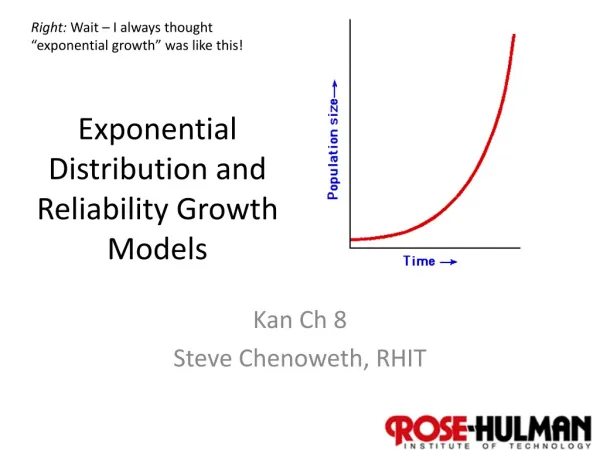
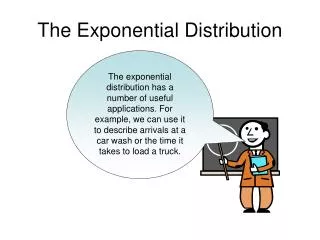
Right: Wait – I always thought “exponential growth” was like this!. Exponential Distribution and Reliability Growth Models. Kan Ch 8 Steve Chenoweth, RHIT. Reliability growth models. Exponential … and more Rayleigh tries to model the whole lifecycle.

E N D
Right: Wait – I always thought “exponential growth” was like this! Exponential Distribution and Reliability Growth Models KanCh8 Steve Chenoweth, RHIT
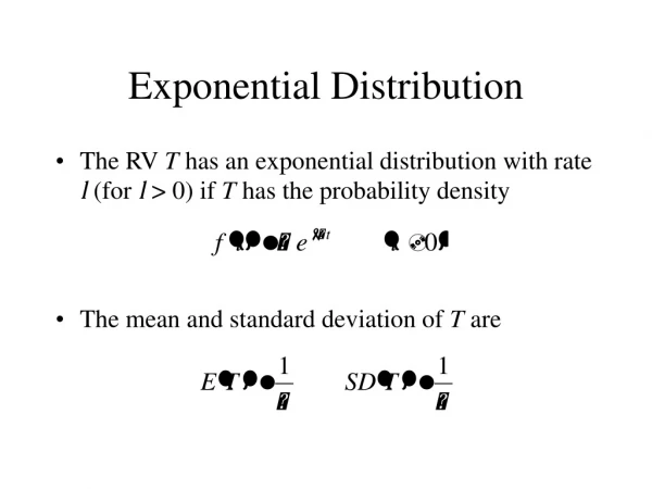
Reliability growth models • Exponential … and more • Rayleigh tries to model the whole lifecycle. • These models, in contrast, are for formal testing phases. • Worth doing because “Defect arrival or failure patterns during such testing are good indicators of the product’s reliability when it is used by customers.” • During formal testing, the software gets more stable, and “reliability grows.”
What do we mean by “reliability”? • More general than often used for large systems, where – • Reliability = MTBF, and • A “failure” is like a system crash. • Instead, here “reliability” = absence of all kinds of measurable faults, including: • Little things not working, and • Features not meeting specs.
And, it works… • Lots of places where this model is known to predict failures over time. • Can estimate defect arrival rates or time between failures. • Kan used for AS/400 studies. • Easy to set up. • A good place to start in modeling testing.
More complex models • Try to fix problems with exponential model. • Generally more complex to set up. • May be harder to get their additional data.
Jelinski-Moranda model • A time between failures model • Assumes – • N software faults at start of testing. • Failures occur purely at random. • All faults contribute equally to cause a failure. • Fix time is negligible. • Fix for each failure is perfect. • Thus, software product’s failure rate improves by the same amount at each fix.
Jelinski-Morandamodel, cntd • So, the “hazard function” • The instantaneous failure rate function • At time ti, which is between failures (i-1) and I, is • Z(ti) = [N – (i – 1)] , where • N = number of defects at beginning of testing, and • is a proportionality constant (not a function). • As each fault is removed, the hazard function decreases in value, and the time between failures increases.
Even messier models • Each of these tries to get rid of some possibly untenable assumption in the previous models. • E.g., in the Goel-Okumoto Imperfect Debugging Model, • Defect fixes are allowed to be imperfect. • Z(ti) = [N – p(i – 1)], where • N = the number of faults at the start of testing, • P = probability of imperfect debugging, and • = the failure rate per fault.
The Delayed S and Inflection S Models • Allow for separate defect detection and defect isolation processes. • The S-shaped curve that results allows for the delay between first failure observation and the time of reporting. • The S-curve results from this delay in reliability growth. • The inflection model also allows for detection dependence – the more we find, the more undetectable failures become detectable.
Criteria for Model Evaluation • Predictive validity • Capability • Quality of assumptions • Applicability • Simplicity Bold = Kan’s preferences.
How to model reliability • Examine the data. • Select the model or several models. • Estimate the parameters for the model. • Obtain the fitted model, by substituting the parameters. • Perform a goodness-of-fit test and assess reasonableness of the model. • Make reliability predictions based on the fitted model.
Steps 2, 3, & 4 2. Picked Exponential Model. • Had used Delayed S and Inflection S Models before, but, • In this data, Kan didn’t notice an increase-then-decrease pattern typical of those models! 3. Used two SAS processes to get constants K and . (See slide 4.) 4. Plugged those into the exponential model.
Step 5 • Used Kolmogorov-Smirnov goodness-of-fit test, to validate the model:
Step 6 • Kan used this model during 4 years worth of testing! • “The projection from this model was very close tto the estimate from the Rayleigh model and to the actual field defect data.”
Test Compression Factor • These tests work best when: • Project is large, • Defect arrival rates tend not to fluctuate much, • The system is not safety-critical (!), and • Environment-specific factors are taken into account. • But, even being this cautious doesn’t mean you can extend the model into customer use (e.g., maintenance)!
What’s different about maintenance? • During testing, the sole purpose is defect detection and removal. • Test cases are maximized for defect detection. • Defect arrivals – usually much higher. • Customer, in contrast, takes time to find defects! • Defect arrivals may be much more spread out. • The difference between these = the “compression factor.”
Estimating Total Defects • Use reliability models and, • Historical patterns for projecting into field use.
Fast vs Slow Ramp-up • Large systems and O/S’s – slow (3 years) • Typical apps – fast (2 years)
Conclusion on ramp-ups • Use your own historical data to estimate for new products. • Kan recommends a nonparametric method • Like 3-point moving average • To smooth the data.
Recommendations for small projects • For Ch 7 - Rayleigh can work, but requires people with the modeling expertise. • From Ch 6 – Use a test effectiveness metric, validate with prior projects. Then, • For Ch 8 – Gather data, etc., as described on p 220. • Pick a simple metric (in terms of both data needed and complexity to validate). • Interval estimating is easier. • Cross-validate results across projects, if comparable. • Know your assumptions!