Download
1 / 46
460 likes | 544 Views
Control of a Lake Network Invasion: Bioeconomics Approach. Alex Potapov, Mark Lewis, and David Finnoff* Centre for Mathematical Biology, University of Alberta. *Department of Economics and Finance, University of Wyoming. Great Lakes Invasion by Alien Species. Rusty crayfish. Zebra Mussels.

E N D
Control of a Lake Network Invasion: Bioeconomics Approach Alex Potapov, Mark Lewis, and David Finnoff* Centre for Mathematical Biology, University of Alberta. *Department of Economics and Finance, University of Wyoming
Great Lakes Invasion by Alien Species Rusty crayfish Zebra Mussels Sea Lamprey
Economic Impact: Average Cost to Control Zebra Mussels by Plant Type as of 1995:Hydroelectric facilities $83,000.Fossil fuel generating facilities $145,000.Drinking water treatment facilities $214,000.Nuclear power plants $822,000.
Damage to Recreation, Change in Ecosystems Beaches covered by shells, smell, cleared water, less sport fish
Zebra mussel spread 1988 2003
How do invaders spread? • To the Great lakes – various ways, mainly by ships in ballast water. • Within the lake system – naturally • To land lakes and between them – mainly through fishing and boating equipment. • Prevention – equipment washing…
20 researchers from 5 universities: D. Lodge and Gary Lamberti (U Notre Dame), M. Lewis (U Alberta), H. MacIsaac (U Windsor), J. Shogren and D. Finnoff (U Wyoming), Brian Leung (McGill) • 5 year project • Collaborative project between biologists, economists and mathematicians • http://www.math.ualberta.ca/~mathbio/ISIS
Analysis using optimal control theory • Clark C.W. Mathematical Bioeconomics. The optimal management of renewable resources. 1990. • Van Kooten G. C. and Bulte E. The Economics of Nature, 2000 . • Main idea: • Model an ecological system as a dynamical system • Include human activity and costs/benefits • Determine the optimal harvesting/management via optimal control theory
Population level Losses/changes Prevention/ Control Expenses Costs/Benefits Introduction Transportation Dispersal Optimization Invader dynamics + costs/benefits optimization (integrative bioeconomic models)
General invasion model with control Model includes dynamics of the invader in the lake ui, possible controls, minimization of costs (or maximizing benefits) Minimize costs or maximize benefits
Macroscopic model for invasion spread Invasion is described in terms of proportion of infected lakesp=NI/N. Invader propagules are transported from lake to lake by boats (intensity A1), probability of survival A2, increase in number of infected lakes t=Np during t is (N–NI)NItA1A2,
Invader Control Prevention effort at infected and uninfected lakes: x and s (effort/lake/time). Probability of propagule escaping treatment at infected lake is a 1, and at uninfected lake is b 1 . Washing efficiency 1–a, and1–b. Assume effects of two successive prevention treatments are independent: a(x1+x2)=a(x1)a(x2) Dynamic equation for proportion of lakes invaded:
Costs Invasion cost: g ($/lake/time) – decrease in benefits or increase in costs Prevention cost: wx at invaded lakes ws at uninvaded lakes Total invasion cost/lake:
Discounting and optimality Total cost during time interval 0 t T: Cost functional Discounting function Dynamical equation for proportion of lakes invaded p(t) (optimization constraints) Optimal control problem: minimize J by choosing x(t)and s(t)0 tT
Maximum Principle Goal: maximizeH (Hamiltonian) Dynamical equation for shadow price m(t) with terminal condition Dynamical equation for proportion of lakes invaded p(t) with initial condition Optimality (max in x, s) conditions at any 0t T
Optimality conditions Three types of control 1. Donor control 2. Recipient control 3. No control
Non-overlapping control regions x-control s-control No control p0 Finish here at time t=T, p=pe The current value Hamiltonian H is maximized by x=x*, s=s* Start here at time t=0 When there is no discounting (r=0), solution can be calculated analytically from
Terminal time specifies optimal trajectory Proportion infected lakes T small: No control T intermediate:Donor, then No control T large: Donor, then Recipient then No control Shadow price Donor control Recipient control Terminal time For any given T, there exists and optimal trajectory T T T pe pe pe 1 Proportion infected lakes
Two different phase plane representations (p- plane, control-p plane) Proportion infected lakes Shadow price—proportion infected phase plane Shadow price Donor control Recipient control Donor control Recipient control Control costs—proportion infected phase plane Control costs Proportion infected lakes
Effect of the discount rate Proportion infected lakes Solid line: No discounting (solution is calculated analytically) Dashed line: With discounting (solution must be calculated numerically) Shadow price Donor control Recipient control Recipient control Donor control Control costs Proportion infected lakes
Outcomes with and without discounting Without discounting Control levels Proportion infected lakes With discounting Proportion infected lakes Control levels
No control is optimal Control efficiency k=k1=k2 is varied. Thick solid — x(t), thick dashed — s(t), thin solid — p(t), thin dashed — uncontrolled p(t), A=1, p0=0.3, g=0.5, r=0, T=50,.
Conclusions-1 • We can delay invasion but not stop it. • Goal is to delay invasion so as to increase net benefit from a bioeconomic perspective. • Problem can be analyzed using phase plane methods. • Three main strategies for controlling invaders: Donor control, recipient control, no control. Switching occurs between strategies as the invasion progresses. • Short (e.g., political) time horizons can yield no control as optimal. • Control strategies are sensitive to discounting. Discounting reduces early investment in control and allows invasion to progress quickly.
Model extension: eradication C is linear in h, bang-bang control: h=0 or h=hmax.
New kind of solution: complete eradication If we eradicate invader by some moment t1, then for t>t1 there are no losses and no costs. New formulation: free terminal time, fixed end state p=0, and hence s=0. Different boundary condition
Variety of solutions: isochrones view Isochrone = set of all initial states (p,) such that (T)=0 p0 Complete eradication trajectory Beginning of optimal trajectory Beginning of suboptimal trajectory Eradication is optimal Isochrone with appropriate T New effect: several locally optimal solutions. Complete eradication is the optimum only for big enough T.
Terminal value: beyond the control horizon At t=T the ecosystem remains and still can bring benefits, must have some value V(pe). Then it is necessary optimize cost+terminal value. Let a system with invasion level p under controls x(t) produces benefits with a rate W(p,x), then we need How to define VT(p(T))?No agreement on this at present.
Invariant terminal value Let us define V through infinite horizon problem. p(0)=p0. Define Value = present cost of maximum future benefits under optimal management Then solution of a finite time horizon T optimal control problem with terminal cost V(pe) coincides with x(t) on (0,T) (x(t) does not depend onT). Can be formulated in terms of minimizing future costs under
A solution of an infinite-horizon problem (IHP) ends at an invariant set of the dynamical system. Theorem. Let the solution of IHP {x(t),p(t)} exists and is unique for each p0=p(0) and the corresponding invariant end-state. Then optimal control xT(t) for finite-horizon problem with the terminal value V(p(T)) and the same p0xT(t)=x(t) on (0,T). Either xT(t)=x(t), 0<t<T,p(T)=p(T), or a contradiction
Proof: suppose p(T)p(T), then • VT>V, then x(t) is not optimal • VT=V, then x(t) is not unique • VT<V, then x(t) is not optimal • xT(t)=x(t), 0<t<T (optimality principle)
Example: no eradication r=0.01 r=0.07
Example: with eradication No eradication at the end r=0.03 r=0.01 Complete eradication Optimal trajectory Suboptimal trajectory r=0.10
Implications of terminal value for the problem with explicit spatial dependence • Optimal control problem – system of 2N equations; • Infinite-horizon problem – only steady states are important; at small discount – look for the best steady state; • May be a considerable simplification: first study steady states, then choose a best way to them
Accounting for Allee effect • Allee effect – population cannot grow at low density • Cannot be integrated into the macroscopic model • Single lake description
Allee effect with external flow Weak external flow, w<|Fmin|, population still goes extinct at small u; Strong external flow, w>|Fmin|, population grows from any u No external flow, population goes extinct at small u
Explicit spatial model with Allee effect Optimal invasion stopping: find optimal spatial controls distribution that keeps flow below critical at uninvaded lakes We can look for the optimal place to stop the invasion
Example: Linearly ordered lakes, Bij=B(|i–j|) Numerical solution gives spatial distribution of controls Bij=B0exp(–|i–j|) Bij=B0/ (1+(|i–j|)2)
Conclusions-2 • Eradication of the invader can make the problem of finding optimal control more complicated and gives new strategies; • Terminal value through infinite-horizon problem reduces analysis to steady states and trajectories leading to them – a considerable simplification of analysis, especially for high-dimensional problems, + more transparent management recommendations; • Allee effect allows to stop invasion without eradication; accounting for the terminal value leads to the natural problem of optimal invasion stopping
Acknowledgements • ISIS project, NSF DEB 02-13698 • NSERC Collaboration Research Opportunity grant.. References A.B. Potapov, M.A. Lewis, D.C. Finoff. Optimal Control of Biological Invasions in Lake Networks. Journal of Economic Dynamics and Control, 2005(submitted). D.C. Finoff, M.A. Lewis, A.B. Potapov. Optimal Control of Biological Invasions in Lake Networks., 2005(in preparation). A.B. Potapov, M.A. Lewis. Optimal Spatial Control of Invasions with Allee Effect., 2005(in preparation).
Influence of invasion losses per lake g on the optimal control policy
Influence of control time horizon T on the optimal control policy
Influence of initial proportion of infected lakes on the optimal control policy
Influence of discounting rate r on the optimal control policy