Download
1 / 29
290 likes | 407 Views
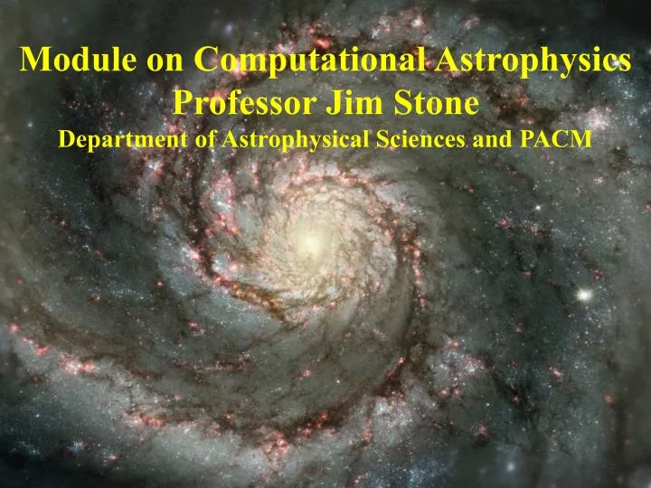
Module on Computational Astrophysics Professor Jim Stone Department of Astrophysical Sciences and PACM. Module on Computational Astrophysics. Jim Stone Department of Astrophysical Sciences 125 Peyton Hall : ph. 258-3815: jmstone@princeton.edu www.astro.princeton.edu/~jstone.

E N D
Module on Computational Astrophysics Professor Jim Stone Department of Astrophysical Sciences and PACM
Module on Computational Astrophysics Jim Stone Department of Astrophysical Sciences 125 Peyton Hall : ph. 258-3815: jmstone@princeton.edu www.astro.princeton.edu/~jstone Lecture 1: Introduction to astrophysics, mathematics, and methods Lecture 2: Optimization, parallelization, modern methods Lecture 3: Particle-mesh methods Lecture 4: Particle-based hydro methods, future directions
When is computation needed in astrophysics? • Calculating the orbits of planets over billions of years • Requires very accurate N-body methods • Stellar structure and evolution • Requires ODE solver, numerical linear algebra, hydrodynamics • Formation of stars and planets • Hydrodynamic and MHD solvers, N-body methods • Dynamical evolution of star clusters • Very fast N-body methods • Formation of galaxies • Very fast N-body methods, hydrodynamics • Data analysis and image processing (astronomy) • Numerical linear algebra, pattern recognition, data mining
Thus, computational methods of interest to astronomers and astrophysicists are: • N-body methods • ODE solvers • Numerical linear algebra • Hyperbolic, parabolic, elliptic PDE solvers • Image processing, data mining and analysis We can’t cover it all! We have to focus on one topic:
N-body algorithms Why N-body methods? • Allow one to study interesting problems • Physics is simple • Mathematics is simple (but not too simple) • Computational methods are complex (but not too complex) • Methods are applicable in other disciplines (e.g. plasma physics, molecular dynamics) Let’s look at some examples of the application of N-body methods to problems in astrophysics…
Example 1. Orbits of solar system bodies from Doug Hamilton’s webpage Solar System Viewer
Example 2: Stellar dynamics at the galactic center
Example 3: Stellar dynamics in a globular cluster
Example 3. (continued) Movie from Frank Summers, AMNH
Example 4. Stellar dynamics during collision of two galaxies
Example 4. (continued) Calculation by Chris Mihos, Vanderbilt U.
Example 5: Formation of structure in the Universe Evolution of the Universe is an initial value problem The past: temperature fluctuations 300,000 years after the Big Bang WMAP
The present:distribution of galaxies near the Milky Way today (14 billion years after Big Bang)
Example 5: Formation of structure is computed by N-body simulations (particles represent dark matter) Movie by Andrey Kravtsov, U. Chicago
Example 5: (continued) Zoom-in on formation of cluster of galaxies
Example 6. Dynamics of galaxies during cluster formation Movie by John Dubinski, U. Toronto
How are these results computed? Motion of individual particles given by Newton’s Laws Forces computed from Newton’s Law of Gravity “Just” have to solve two coupled ODEs, plus evaluate forces.
Introduction to mathematics of the N-body problem. We will use numerical methods to get solutions to the equations of motion. Useful to understand mathematical properties of solutions. For N=2, solution can be computed analytically (two-body problem). Total momentum p = m1v1 + m2v2 Rate of change of p: dp/dt = m1dv1/dt + m2dv2/dt = F1 + F2 But F1 = -F2, --> dp/dt = 0 --> p = const. So particles move around a common point (the Center of Mass), which moves at a constant velocity.
C of M R Two-body problem (continued) Can show motion of particles follows Kepler’s Third Law R = distance between particles P = period of orbit
For N=3, no analytic solution possible (!!) Example of orbits in a 3-body encounter
For N=3, no analytic solution possible (!!) Approximate solutions are possible in certain limiting cases, e.g. when one particle is much less massive than other two. BUT, certain constraints still apply (useful as diagnostics): Total energy conserved Angular momentum conserved Total momentum conserved, so center of mass moves at constant velocity (providing 6 more constraints).
For continuum approximations apply. Rather than solving for the position of each particle individually, instead compute the evolution of the phase space density: f (x, v, t) At any instant in time, each particle is represented by a point in the 6-dimensional space (x, v). There are so many particles, this space is filled with points. f represents the density of points in this space, and it evolves in time according to the Boltzmann equation: Hard part is evaluating the collision term. Common to use the Fokker-Planck approximation. Continuum methods work well for dense stellar systems, but not when single particle interactions (binaries) are important.
Timescales in N-body problems. Most fundamental is the crossing-time. Consider a star cluster of radius R which contains N stars of mass m By the virial theorem, for a system in equilibrium, the sum of kinetic and potential energies for a single star is: So For N=104, m = 0.5 solar masses, R = 4 pc, tcross = 5 million years But age of cluster is about 10 billion years >> tcross In addition, orbital time of binaries in cluster can be << tcross Multi-timescale problem
Computational Tasks Setup distribution of N particles Compute forces between particles Evolve positions using ODE solver Display/analyze results
1. Setup initial distribution of particles Can be complex for large N Need realistic model of mass distribution in cluster, galaxy, etc.
2. Computing Forces between particles. Magnitude of force on ith particle This diverges as distance between particles --> 0 Can cause very small time steps. Solution is to use a softened potential e = softening parameter Physically, this eliminates the formation of binaries with r < e Hard binaries (very small separation) are an important source of energy in clusters; this means e should be as small as possible
Direct summation is most straightforward method of evaluating F But, number of operations scales as N(N-1)/2 Severly limits number of particles, usually N < 104 Motivates finding more efficient techniques (more later)
3. Evolve positions using ODE solver Could use any ODE solver (e.g. Runge-Kutta, Burlisch-Stoer, …) Must balance accuracy versus efficiency Need many particles to capture dynamics correctly, which can be just as important as the accuracy of any one particle orbit (except for planetary orbits, when N small). Perhaps most popular method is leap-frog.
n-1 n-1/2 n n+1/2 n+1 time x, F v x, F v x, F Leap-frog scheme Define positions (x) and forces (F) at time level n velocities (v) at time level n+1/2 Then, for ith particle To start integration, need initial x and V at two separate time levels. Specify x0 and v0 and then integrate V to Dt/2 using high-order scheme