Download
1 / 29
290 likes | 403 Views
QuickYield: An Efficient Global-Search Based Parametric Yield Estimation with Performance Constraints. Fang Gong 1 , Hao Yu 2 , Yiyu Shi 1 , Daesoo Kim 1 , Junyan Ren 3 , and Lei He 1. 1 University of California, Los Angeles, Los Angeles, US 2 Nanyang Technological University, Singapore

E N D
QuickYield: An Efficient Global-Search Based Parametric Yield Estimation with Performance Constraints Fang Gong1, Hao Yu2, Yiyu Shi1, Daesoo Kim1, Junyan Ren3, and Lei He1 1University of California, Los Angeles, Los Angeles, US 2Nanyang Technological University, Singapore 3State Key Lab of ASIC, Fudan University, Shanghai, China Presented by Fang Gong
Outline • Introduction • Algorithms • Experimental Results • Conclusions
Need of Fast Yield Estimation • Process Variation is an major source of yield loss • lithography, CMP and etc. • Threshold voltage, timing delay, and etc. • Larger Variation with scaling leads to lower Yield Rate. * Data Source: Dr. Ralf Sommer, DATE 2006, COM BTS DAT DF AMF; It is important to predict the Yield accurately.
Monte Carlo Simulation • Generate huge number of parameter samplings according to probability distribution; • Perform simulation to find performance merit of interest; • Compare with performance constraint to identify success points in the parameter space. Monte Carlo method is highly time-consuming! Fast Yield Estimation becomes necessary!
Success region Yield Boundary ƒm(γp)=ƒworst Yield Boundary in Parameter Space • Parameter space is the space bounded by the min and max of all process parameters around nominal values(blue square); • Yield Boundary separates success region from fail region; • success region where parameters lead to acceptable performance. • ƒmis the performance merit of interest; • γp is the process parameters subject to random variations. • ƒworstis the worst-case performance that can be accepted.
Success region Fail region Definition of Yield by Boundary Yield = Ssuccess / Sentire • Ssuccess : the region where parameters lead to successful performance. • Sentire : the entire space that variable parameters can be reached around their nominal values (blue square). • In the parameter domain, all parameters follow uniform distributions. Other distributions can be transformed into uniform ones*. *Luc Devroye. Non-Uniform Random Variate Generation. New York: Springer-Verlag, 1986.
ƒm(γp)=ƒworst Framework of Existing Methods (1) • Any circuit can be described by differential algebraic equation (DAE) system → performance surface • Performance constraints → Constraint Plane • Yield Boundaryis the projection of intersection boundary of these two surfaces in the parameter domain. Local searches in existing work
Framework of Existing Methods (2) Perform SPICE simulation with initial parameters; Compare performance merit with performance constraints; If not satisfied, select new parameters and repeat. p2 p1 p0 Multiple simulations for one point at boundary/surface. How to locate the yield boundary in the parameter space with global search? Reference: P. Cox, P. Yang, and P. Chatterjee, IEDM’83; S. Srivastava and J. Roychowdhury, CICC’07; C. Gu and J. Roychowdhury, ASPDAC2008
Outline Introduction Algorithms Global-Search based Surface Building Global Search for Surface Point Experimental Results Conclusions
Surface Building: Init Step (1) • Calculate Intersection points (P01 and P02) at each parameter axis; • By connecting two points(P01 and P02) , the boundary can be estimated with piecewise linear approximation. Linear Approximation to the Boundary/Surface
Y YP04 YP03/YP05 XP05 X XP03/XP04 Surface Building: Refinement (2) • Start from the middle point (P03)of line (P01P02)to find additional surface points P04 andP05 • XP03 = XP04, YP03=YP05 • Treat YP04 and XP05 as the unknown parameters γp; • Solve the augmented system for unknowns. One-time simulation for one boundary point!
Surface Building: Refinement (2) • Refine the yield estimation by refining the linear approximation.
Existing Method QuickYield Key Idea of QuickYield
Comparison to Existing Work • QuickYield performs one simulation for each surface point. • Yield Estimation via Nonlinear Surface Sampling (YENSS) • locally searches along the tangent direction of performance surface to locate one surface point. • Several simulations are performed to locate one single surface point. • Search requires expensive sensitivity analysis. * C. Gu and J. Roychowdhury, “An efficient, fully nonlinear, variability-aware non-monte-carlo yield estimation procedure with applications to sram cells and ring oscillators,” in ASP-DAC ’08, 2008.
Outline Introduction Algorithms Global-Search based Surface Building Global Search for Surface Point Experimental Results Conclusions
Representation of Global Search • Parameter finding is initially used for device optimization, and we will discuss its application in yield estimation. • Original circuit in differential algebra equation (DAE) representation: • Integrating the performance constraint can be integrated into DAE system as: The nonlinear system can be solved with Newton-Raphson Iterations.
Jacobian Matrix in Newton Method • For DC analysis: • For Periodical Steady State (PSS) Analysis
Outline • Introduction • Algorithms • Experimental Results • Conclusions
Schmitt Trigger • Consider channel widths of Mn1 and Mp2 as variational parameters. • 30% variations from nominal values; • Other process parameters can be handled in the same way. • Performance Constraint: • Lower switching threshold VTL as performance merit; • When the input VTL is 0.4V and the output is pre-charged to Vdd, the output VOUH should be greater than 1.7V
Results • QuickYield can achieve only 0.4% error compared with Monte Carlo method, and gain 349X speedup. QuickYield
3-stage Ring Oscillator • Performance Constraint:oscillator period • Determined by the delay of inverters; • Nominal Tnorm is 7.2028ns; • Performance Constraint: period variation ΔT should be within ± 2.5% of nominal Tnorm. • MOSFETs in the first stage have channel width variations with 3σ=40% perturbation range (Gaussian distribution)
Accuracy • Two performance constraints two yield boundaries • T> Tnorm * (1- 0.025) • T< Tnorm * (1+ 0.025) Tmin (QuickYield) Tmax (QuickYield)
Runtime • YENSS results are normalized with respect to Monte Carlo method from published paper. • QuickYield can obtain 519X speedup over Monte Carlo at a similar accuracy.
Scalability • The scalability of QuickYield with the number of Surface Points: • Runtime increases linearly while the yield converges quickly.
High-dimensional Case • The load capacitance C1 has been introduced random variation to increase the complexity. • QuickYield can achieve as low as 0.6% error.
Runtime • QuickYield can be up to 267X faster than MC and 4.6X faster than YENSS.
Outline • Introduction • Algorithms • Experimental Results • Conclusions
Conclusions and Future Work • A fast algorithm, QuickYield, was proposed: • Augmenting DAE system with performance constraint. • Locating the yield boundary with global search by solving the augmented system. • Up to 519X faster than MC and up to 4.7X than YENSS, while keeping the same accuracy. • Future work: • handle more variables and multiple performance constraints simultaneously.