Download
1 / 27
270 likes | 382 Views
Deterministic Random Walk Preconditioning for Power Grid Analysis. Jia Wang Electrical and Computer Engineering Illinois Institute of Technology Chicago, Illinois, United States November, 2012. Agenda. Power Grid Analysis Overview of IC and Stochastic Preconditionings

E N D
Deterministic Random Walk Preconditioningfor Power Grid Analysis Jia Wang Electrical and Computer Engineering Illinois Institute of Technology Chicago, Illinois, United States November, 2012
Agenda • Power Grid Analysis • Overview of IC and Stochastic Preconditionings • Deterministic Random Walk Preconditioning • Experimental Results
The Key Problem Solve the following equations for the vector x Properties of the LHS matrix A Square, sparse, nonsingular, symmetric Diagonally dominant with nonpositive off-diagonal elements Imply symmetrix M-matrix and S.P.D. Arise from many power grid analysis problems DC analysis Transient simulation w/o mutual inductances after discretization [Chen and Chen DAC'01] 3
Challenges and Solutions • The size of the problem is extremely large. • Recent public IBM power grid benchmarks can have more than 1 million variables. • Storage of A is not a concern as A is sparse. • Direct method: Cholesky factorization • The factor, though remains relatively sparse via minimum degree orderings, could still require tremendous storage. • It is a waste of effort to compute the factor if it is used only a few times, e.g. for DC analysis. • Fast approximations • Exploit certain aspect of power grid, e.g. mesh structure • Desirable if accuracy could be traded off for solution time • Iterative methods, e.g. based on Conjugate Gradient • Hierarchical analysis
Iterative Methods Preferred when accuracy becomes a concern. e.g. for recent power grid contests (TAU'11, TAU'12) Preconditioner matters: classical ones or fast approximators Approximating Factors Incomplete Cholesky (IC) [Chen and Chen DAC'01] Stochastic preconditioning [Qian and Sapatnekar ICCAD'05] Multigrid w/ Successive Over Relaxation [Zhong and Wong ICCAD'05] on GPU [Feng et al. TCAD'11] Algebraic multigrid (AMG) [PowerRush Yang et al. ICCAD'11] Many others Domain decomposition [Sun et al. ICCAD'07], Sub-circuit [Chou et al. ICCAD'11], Possion solver [Yang et al. ICCAD'11], Support graph [Zhao et al. ICCAD'11] 5
Iterative Methods Preferred when accuracy becomes a concern. e.g. for recent power grid contests (TAU'11, TAU'12) Preconditioner matters: classical ones or fast approximators Approximating Factors Incomplete Cholesky (IC) [Chen and Chen DAC'01] Stochastic preconditioning [Qian and Sapatnekar ICCAD'05] Multigrid w/ Successive Over Relaxation [Zhong and Wong ICCAD'05] on GPU [Feng et al. TCAD'11] Algebraic multigrid (AMG) [PowerRush Yang et al. ICCAD'11] Many others Domain decomposition [Sun et al. ICCAD'07], Sub-circuit [Chou et al. ICCAD'11], Possion solver [Yang et al. ICCAD'11], Support graph [Zhao et al. ICCAD'11] fastest convergence among explicit preconditioners fastest for DC analysis on IBM benchmarks 6
Stochastic Preconditioning • Utilize random walks on the power grid • Fast approximation for solutions [Qian et al. DAC'03] • Preconditioning with approximated factors [Qian and Sapatnekar ICCAD'05] • Advantage: fast convergence • We observed that the residue can be reduced by half per PCG iteration with less than 2X non-zeros in the approximated factors compared to those in A. • Disadvantage: long setup time • Need to perform actual random walks via Monte Carlo simulations to generate the preconditioner • Remain relatively slow despite speed-up techniques [Qian and Sapatnekar '08] Can we speed-up the setup process w/o affecting preconditioner quality?
Hierarchical Analysis Divide-and-conquer [Zhao et al. TCAD'02] Partition the whole grid into local and global ones Approximate the Schur complement as the exact one is usually dense Closely related to domain decomposition methods Hierarchical Random Walks Use random walks to approximate the Schur complement Reuse local random walks at pre-defined partitioning interfaces [Qian et al. TCAD'05] Form the hierarchy by random sampling instead of partitioning [Li DAC'05] Can we use hierarchical random walks to speed-up stochastic preconditioning? Not trivial since factorizing the approximated Schur complement may affect preconditioner quality 8
Our Contributions Design an algorithm to estimate random walk probabilities in a deterministic manner In order to build the preconditioner Exploit probabilities of previous random walks to avoid expensive Monte Carlo simulations, and to eliminate all of them in a simplified setting Generate preconditioners with similar quality as stochastic preconditioning in less time Compete with AMG-PCG for DC analysis Potentially efficient for transient simulations when direct method is prohibitive due to storage requirement In some sense, we implicitly factor the Schur complement w/o explicitly approximating it first. Similar to traditional incomplete factorizations 9
Agenda Power Grid Analysis Overview of IC and Stochastic Preconditionings Deterministic Random Walk Preconditioning Experimental Results 10
Incomplete Cholesky Factorization The exact root-free Cholesky factorization Incomplete Cholesky [Meijerink and van der Vorst '77] Correctness guarantee for M-matrix [Manteuffel '80] The systematic difference could contribute to slow convergence for large problems. Cannot decrease dk,k and li,k w/o affecting the guarantee 11
Matrix, Graph, and Random Walks • Construct a graph G from A • Edges in G represent non-zeros in A. • Edges from/to an extra vertex represent row/column sums. • Define a random walk game on G • The transfer probability is propotional to the edge weight. • e.g. from 1, 1/3 chance to transfer to 2 or 3 or 4 • Consider random walks starting at k, passing vertices no more than k, and ending at i>k • e.g. walks like 3,1,2,1,4 but not 3,1,4,1,4
Stochastic Preconditioning • Random walks vs. root-free Cholesky factorization • Ek is the expected times those random walks pass k. [Qian and Sapatnekar'08] • One can perform Monte Carlo simulations to compute Cholesky factorizations! • No error accumulation/systematic difference as in IC • Many properties of D and L can be easily preserved. • Diagonal elements of D are positive. • Off-diagonal elements of L are nonpositive. • L is column-wise diagonally dominant. • Length of the random walks cannot be bounded. • e.g. 3,1,2,1,2,1,2,...,1,4, even worse if the edge from 1 to 2 has much larger weight.
Agenda Power Grid Analysis Overview of IC and Stochastic Preconditionings Deterministic Random Walk Preconditioning Experimental Results 14
Decomposition of Random Walks • If we can decompose an arbitrarily long walk into a bounded number of sub-walks, • We may be able to bound the worst-case Monte Carlo simulation time. • We may even be able to reduce the average Monte Carlo simulation time. • Exclude walks returning to the starting point • Walks like 3,1,2,1,3,1,2,1,3,..., would be difficult to decompose. • Leverage monotonicity • Once walks returning to the starting point are excluded, we may construct a walk starting at k using walks starting at j<k. • Total number of sub-walks are bounded as ending points are now monotonically increasing.
Excluding Returning Walks Consider the first time a walk starting at k returns to k. The walk may never return to k and thus all internal vertices are less than k. Or, the walk has to travel vertices less than k before returning to k for the first time. For probabilities, we have The same reasoning can be applied to the expectation. 16
Monotonic Decomposition Consider the second vertex j in the walk starting at k but not returning to k e.g. 3,5 or 3,1,2,1,2,1,4 Let pj be the probability of this single transfer step. We may consider more steps, see paper for details. If j>k, then the walk should stop here. If j<k, then the remaining part of the walk can be decomposed monotonically. e.g. decompose 1,2,1,2,1,4 into 1,2 and 2,1,2,1,4 The probabilities can be calculated from those walks starting at a vertex less than k. 17
Deterministic Random Walk We don't need Monte Carlo simulations any more. The computation of probabilities can be simplified. 18
Deterministic Random Walk We don't need Monte Carlo simulations any more. The computation of probabilities can be simplified. Or, even simpler for q representing the vector of the above common expression and LHS probabilities. A partial forward substitution Compute L column by column, just like IC. 19
The DRW Algorithm The forward substitution should be done in a sparse manner using the algorithm proposed by Gilbert and Peierls. Correctness is guaranteed by choosing a vertex ordering that ensures qk<1 and a proper function f. 20
Implementation Details Vertex ordering Reverse Cuthill-McKee ordering (RCM) Guarantee qk<1 and being memory friendly Dropping and compensation scheme f Globally specify a bound for number of fill-ins Keep all entries larger than a given threshold Keep the largest few entries until per-column bound is met Compensate the dropped entries by scaling up the remaining entries accordingly Differences from an IC preconditioning algorithm with similar dropping scheme DRW only uses L while IC uses both D and L. DRW usually visits more columns in L via forward substitutions than IC to compute the next column. Compensation of L is not allowed in IC for its correctness. 21
Agenda Power Grid Analysis Overview of IC and Stochastic Preconditionings Deterministic Random Walk Preconditioning Experimental Results 22
DC Analysis on IBM Benchmarks Conjugate Gradient with DRW preconditioners Running times are measured on a 64-bit Linux workstation with a 2.4GHz Intel Q6600 processor and 8GB memory. Preconditioners have the same size (# of non-zeros) as A. PowerRush running times are obtained by scaling those from [Yang et al. ICCAD'11].
Detailed Comparisons • Sizes of all the preconditioners are 1.7 times of A. • All results are the averages of 100 random RHS vectors. • IC uses the same vertex ordering and dropping scheme as DRW, but does not compensate for dropped entries. • Stochastic preconditioning uses a different ordering than RCM, which adversely affects PCG solution time.
Impacts of Memory Usage • For IBM DC benchmarks, DRW can be both memory and running time efficient at the same time. • Highly-optimized implementation (CHOLMOD) of direct method is very efficient once a factorization is obtained. However, it consumes a lot of resource for setup and storage.
Conclusion & Future Work • By estimating random walk probabilities in a deterministic manner, we avoided costly Monte Carlo simulations in building a high quality preconditioner. • Our proposed techniques could be extended to handle asymmetric matrices and matrices with positive off-diagonal elements. • We now have an updated version of the DRW algorithm that can accept any vertex ordering, while remaining correct. • This enables us to apply orderings like AMD when RCM is not suitable, e.g. for highly-coupled IBM transient simulation benchmarks published at TAU'12.