Download
1 / 36
420 likes | 642 Views
Supply and Demand. The Supply Curve The supply curve shows how much of a good producers are willing to sell at a given price, holding constant other factors that might affect quantity supplied This price-quantity relationship can be shown by the equation:. S. P 2. The supply curve slopes

E N D
Supply and Demand • The Supply Curve • The supply curve shows how much of a good producers are willing to sell at a given price, holding constant other factors that might affect quantity supplied • This price-quantity relationship can be shown by the equation: Chapter 2: The Basics of Supply and Demand
S P2 The supply curve slopes upward demonstrating that at higher prices, firms will increase output P1 Q1 Q2 Supply and Demand The Supply Curve Graphically Price ($ per unit) Quantity Chapter 2: The Basics of Supply and Demand
S S’ P1 P2 Q0 Q1 Q2 Supply and Demand Change in Supply • The cost of raw materials falls • At P1, produce Q2 • At P2, produce Q1 • Supply curve shifts right to S’ • More produced at any price on S’ than on S P Q Chapter 2: The Basics of Supply and Demand
Supply and Demand • The Demand Curve • The demand curve shows how much of a good consumers are willing to buy as the price per unit changes holding non-price factors constant. • This price-quantity relationship can be shown by the equation: Chapter 2: The Basics of Supply and Demand
The demand curve slopes downward demonstrating that consumers are willing to buy more at a lower price D Supply and Demand Price ($ per unit) Quantity Chapter 2: The Basics of Supply and Demand
D D’ P2 P1 Q0 Q1 Q2 Supply and Demand Change in Demand • Income Increases • At P1, purchase Q2 • At P2, purchase Q1 • Demand Curve shifts right • More purchased at any price on D’ than on D P Q Chapter 2: The Basics of Supply and Demand
S The curves intersect at equilibrium, or market- clearing, price. At P0the quantity supplied is equal to the quantity demanded at Q0 . P0 D Q0 The Market Mechanism Price ($ per unit) Quantity Chapter 2: The Basics of Supply and Demand
Price ($ per unit) S Surplus P1 Assume the price is P1 , then: 1) Qs : Q2 > Qd : Q1 2) Excess supply is Q2 – Q1. 3) Producers lower price. 4) Quantity supplied decreases and quantity demanded increases. 5) Equilibrium at P2Q3 P2 D Quantity Q1 Q3 Q2 The Market Mechanism Chapter 2: The Basics of Supply and Demand
Price ($ per unit) S Assume the price is P2 , then: 1) Qd : Q2 > Qs : Q1 2) Shortage is Q2 – Q1. 3) Producers raise price. 4) Quantity supplied increases and quantity demanded decreases. 5) Equilibrium at P3, Q3 P3 P2 Shortage D Quantity Q1 Q3 Q2 The Market Mechanism Chapter 2: The Basics of Supply and Demand
D D’ S S’ P2 P1 Q1 Q2 Changes In Market Equilibrium • Income Increases & raw material prices fall • The increase in D is greater than the increase in S • Equilibrium price and quantity increase to P2, Q2 P Q Chapter 2: The Basics of Supply and Demand
Prices fell until a new equilibrium was reached at $0.26 and a quantity of 5,300 million dozen S1970 S1998 $0.61 $0.26 D1970 D1998 5,300 5,500 Example 1: Market for Eggs P (1970 dollars per dozen) Q (million dozens) Chapter 2: The Basics of Supply and Demand
S1995 Prices rose until a new equilibrium was reached at $4,573 and a quantity of 12.3 million students $4,573 S1970 $2,530 D1995 D1970 7.4 12.3 Example 2: Market for a College Education P (annual cost in 1970 dollars) Q (millions of students enrolled)) Chapter 2: The Basics of Supply and Demand
Elasticities of Supply and Demand Price Elasticity of Demand • Measures the sensitivity of quantity demanded to price changes. • It measures the % change in the quantity demanded for a good or service that results from a one percent change in the price. • The price elasticity of demand is: Chapter 2: The Basics of Supply and Demand
Elasticities of Supply and Demand Price Elasticity of Demand • The % change in a variable is the absolute change in the variable divided by the original level of the variable. So the price elasticity of demand is also: Chapter 2: The Basics of Supply and Demand
Elasticities of Supply and Demand • Interpreting Price Elasticity of Demand Values 1) Because of the inverse relationship between P and Q; EPis negative. 2) If |EP| > 1, the % change in quantity demanded is greater than the % change in price. We say demand is price elastic. 3) If |EP| < 1, the % change in quantity demanded is less than the % change in price. We say demand is price inelastic. Chapter 2: The Basics of Supply and Demand
The lower portion of a downward sloping demand curve is less elastic than the upper portion. 4 Q = 8 - 2P Ep = -1 2 Linear Demand Curve Q = a - bP Q = 8 - 2P Ep = 0 4 8 Price Elasticities of Demand Price Q Chapter 2: The Basics of Supply and Demand
Elasticities of Supply and Demand Other Demand Elasticities • Income elasticity of demand measures the % change in quantity demanded resulting from a one percent change in income. The income elasticity of demand is: Chapter 2: The Basics of Supply and Demand
Elasticities of Supply and Demand Other Demand Elasticities • Cross price elasticity of demand = the % change in the quantity demanded of one good that results from a one percent change in the price of another good. • The cross price elasticity for substitutes is positive, while that for complements is negative. For example, consider the substitute goods, butter and margarine. Chapter 2: The Basics of Supply and Demand
Elasticities of Supply and Demand Elasticities of Supply • Price elasticity of supply measures the % change in quantity supplied resulting from a 1% change in price. • The elasticity is usually positive because price and quantity supplied are positively related (Higher price gives producers an incentive to increase output) • We can refer to elasticity of supply with respect to interest rates, wage rates, and the cost of raw materials. Chapter 2: The Basics of Supply and Demand
SR Versus LR Elasticities Price Elasticity of Demand • Price elasticity of demand varies with the amount of time consumers have to respond to a price. • Most goods and services: • Short-run elasticity is less than long-run elasticity (e.g. gasoline). People tend to drive smaller and more fuel efficient cars in the long-run • Other Goods (durables): • Short-run elasticity is greater than long-run elasticity (e.g. automobiles). People may put off immediate consumption, but eventually older cars must be replaced. Chapter 2: The Basics of Supply and Demand
SR Versus LR Elasticities Income Elasticities • Most goods and services: • Income elasticity is greater in the long-run than in the short run. For example, higher incomes may be converted into bigger cars so the income elasticity of demand for gasoline increases with time. • Other Goods (durables): • Income elasticity is less in the long-run than in the short-run. For example, consumers will initially want to hold more cars. Later, purchases will only to be to replace old cars. Chapter 2: The Basics of Supply and Demand
SR Versus LR Elasticities Price Elasticity of Supply • Most goods and services: • Long-run price elasticity of supply is greater than short-run price elasticity of supply. Due to limited capacity, firms are output constrained in the short-run. In the long-run, they can expand. • Other Goods (durables, recyclables): • Long-run price elasticity of supply is less than short-run price elasticity of supply. For example, consider the secondary copper market. Copper price increases provide an incentive to convert scrap copper into new supply. In the long-run, this stock of scrap copper begins to fall. Chapter 2: The Basics of Supply and Demand
S’ S Coffee prices are volatile: A freeze or drought decreases the supply of coffee in Brazil P1 P0 Short-Run 1) Supply is completely inelastic 2) Demand is relatively inelastic 3) Very large change in price D Q1 Q0 SR Versus LR Elasticities: Coffee Coffee Price Quantity Chapter 2: The Basics of Supply and Demand
Understanding and Predicting the Effects of Changing Market Conditions • We must learn how to “fit” linear demand and supply curves to market data. • We determine numerically how a change in one variable will cause supply or demand to shift and so affect the equilibrium price and quantity. • Assume the Available Data are: • Equilibrium Price, P* • Equilibrium Quantity, Q* • Price elasticity of supply, ES, and demand, ED. Chapter 2: The Basics of Supply and Demand
Supply: Q = c + dP a/b ED = -bP*/Q* ES = dP*/Q* P* -c/d Demand: Q = a - bP Q* Understanding and Predicting the Effects of Changing Market Conditions Price Quantity Chapter 2: The Basics of Supply and Demand
Understanding and Predicting the Effects of Changing Market Conditions • Let’s begin with the equations for supply and demand, and the elasticities: Demand:QD = a - bP Supply: QS = c + dP Chapter 2: The Basics of Supply and Demand
Understanding and Predicting the Effects of Changing Market Conditions • Note: for linear demand curves, ∆Q/∆P is constant (equal to the slope of the curve). • Substituting the slopes for each into the formula for elasticity, we get: Chapter 2: The Basics of Supply and Demand
Understanding and Predicting the Effects of Changing Market Conditions • Suppose we have values for ED, ES, P*, and Q*, we can then solve for b & d, and a & c. Chapter 2: The Basics of Supply and Demand
Example: The Copper Market • Suppose we want to derive the long-run supply and demand for copper: • The data are: • Q* = 7.5 mmt/yr. • P* = 75 cents/pound • ES = 1.6 • ED = -0.8 Chapter 2: The Basics of Supply and Demand
Price Supply: QS = -4.5 + 16P 1.69 = a/b .75 +.28 = -c/d Demand: QD = 13.5 - 8P Mmt/yr 7.5 Understanding and Predicting the Effects of Changing Market Conditions Chapter 2: The Basics of Supply and Demand
Example 1: Real versus Nominal Prices of Copper 1965 - 1999 Chapter 2: The Basics of Supply and Demand
Declining Demand and the Behavior of Copper Prices • The relevant factors leading to a decrease in the demand for copper are: 1) A decrease in the growth rate of power generation 2) The development of substitutes: fiber optics and aluminum • We will try to estimate the impact of a 20% decrease in the demand for copper. • Recall the equation for the demand curve: Q = 13.5 - 8P Chapter 2: The Basics of Supply and Demand
Real versus NominalPrices of Copper 1965 - 1999 • Multiply the demand equation by 0.80 to get the new equation. This gives: Q = (0.80)(13.5 - 8P) = 10.8 - 6.4P • Recall the equation for supply: Q = -4.5 + 16P • The new equilibrium price is: -4.5 + 16P = 10.8 - 6.4P -16P + 6.4P = 10.8 + 4.5 P = 15.3/22.4 = 68.3 cents/pound Chapter 2: The Basics of Supply and Demand
Example 2: Government Intervention - Price Controls • If the government decides that the equilibrium price is too high, they may establish a ceiling price. • Natural Gas Market: In 1954, the federal government began regulating the wellhead price of natural gas. • In 1962, the ceiling prices that were imposed became binding and shortages resulted. • Price controls created an excess demand of 7 trillion cubic feet. • Price regulation was a major component of U.S. energy policy in the 1960s and 1970s, and it continued to influence the natural gas markets in the 1980s. Chapter 2: The Basics of Supply and Demand
S If price is regulated to be no higher than Pmax, quantity supplied falls to Q1 and quantity demanded increases to Q2. A shortage results. P0 Pmax D Excess demand Q1 Q0 Q2 Effects of Price Controls Price Quantity Chapter 2: The Basics of Supply and Demand
Price Controls andNatural Gas Shortages The Data: Natural Gas Chapter 2: The Basics of Supply and Demand