Download
1 / 38
380 likes | 482 Views
2 nd UK-JAPAN Bilateral and 1 st ERCOFTAC Workshop, Imperial College London. PIV study of fractal grid turbulence. S. Discetti 1 , I. B. Ziskin 2 , R.J. Adrian 2 , K. Prestridge 3 1 DIAS, University of Naples Federico II, Naples (Italy)

E N D
2nd UK-JAPAN Bilateral and 1st ERCOFTAC Workshop, Imperial College London PIV studyoffractalgridturbulence S. Discetti1, I. B. Ziskin2, R.J. Adrian2, K. Prestridge3 1DIAS, UniversityofNaples Federico II, Naples (Italy) 2School for Engineering of Matter, Transport and Energy, Arizona State University, AZ (USA) 3Los Alamos National Laboratory, NM (USA)
Motivation • Multi-scale generated turbulence may lead to exciting new insights into turbulence theory as well as important new industrial applications: • Turbulence generated by injecting energy over a range of length scales; • Uncommon fast turbulence kinetic energy decay, well modeled by a self-preserving single lengthscale decay model (George and Wang, POF, 2009); • About three times higher Reynolds number Reλ than turbulence generated by classical grids. • PIV can be a useful tool to obtain a better understanding of the fluid dynamics of fractal-generated turbulence.
Square space-filling fractal grids • Despite of the geometrical complexity, the grid features are defined by a few parameters: • Lo an to, i.e. length and thickness of the largest square; • RL and Rt, i.e. the scaling factors for the length and the thickness at each iteration (more often the thickness ratio trbetween the largest and the smallest scale is considered as a main parameter).
Experimental setup The grids are tested in a low turbulence level open circuit wind tunnel, with a 1,524mm long and 152.4mm wide square test section. The fractal grid is placed at the inlet of the test section, immediately after the contraction.
Experimental setup ≈50mm Measurement area 385mm 600mm The grids are tested in a low turbulence level open circuit wind tunnel, with a 1,524mm long and 152.4mm wide square test section. The fractal grid is placed at the inlet of the test section, immediately after the contraction.
Particle Image Velocimetry Fig. from Raffel et al., Particle Image Velocimetry – A practical guide, Springer Ed. (2007)
Test procedure • Optical calibration: • Images of a target with equally spaced dots with diameter of 250μm and spacing of 1mm are recorded to determine the magnification map as a function of the physical space coordinates; • Images of the particle distributions are taken simultaneously by two cameras in a pre-processing run to determine via disparity map computation the location of the laser sheet in the physical space to properly set the local magnification. • Image acquisition (5000 samples to ensure satisfactorily statistical convergence) • Image Processing • IW: 32 x 32 pixels (0.63 x 0.63 mm comparable to the laser sheet thickness) with 75% overlap; • Multi-pass iterative window deformation with adoption of weighting windows in cross-correlation to enhance the spatial resolution.
Mean flow features Mean streamwise velocity for tr=13 and ReM=3.5∙103 U [m/s] U [m/s] U [m/s]
Mean flow features Mean streamwise velocity for tr=13 and ReM=3.5∙103
Turbulent fluctuations u2 [m2/s2] tr=13 ReM=3.5∙103 v2 [m2/s2]
Anisotropy of the Reynolds tensor tr=13 ReM=3.5∙103 u2/ v2
Two-point correlation tr=13 ReM=3.5∙103 The longitudinal correlation function changes only slightly moving downstream, suggesting that the integral lengthscale increases with the streamwise coordinate. However, the narrow field of view does not enable to estimate it with good confidence.
Longitudinal and transverse correlation functions tr=13 ReM=3.5∙103 x/x*=0.47 This is not equivalent to the longitudinal two-point correlation function (the velocity component is always the streamwise one).
Longitudinal and transverse correlation functions tr=13 ReM=3.5∙103 x/x*=0.47 This is not equivalent to the transverse two-point correlation function (the velocity component is always the crosswise one).
2nd order structure functions tr=13 ReM=3.5∙103 x/x*=0.47 This is not equivalent to the longitudinal 2nd order structure function (the velocity component is always the streamwise one).
2nd order structure functions tr=13 ReM=3.5∙103 x/x*=0.47 This is not equivalent to the transverse 2nd order structure function (the velocity component is always the crosswise one).
Turbulent kinetic energy decay Space filling square fractal grids are characterized by an unusually fast decay: is it governed by an exponential law or a power law? tr=13 ReM=11.5∙103 B=0.526 C=0.262 R2=0.91 B=-0.481 C=-3.90 R2=0.91
Turbulence decay ReM=3.5∙103 Exponential decay ReM=11.5∙103
Turbulence decay ReM=3.5∙103 Power-law decay ReM=11.5∙103
Turbulence decay ReM=11.5∙103
Turbulence decay ReM=11.5∙103
Turbulence decay - remarks • It is not possible to conclude if the decay law is exponential or a power law by visual inspection or using the correlation factor of the fitting law; • More confidence in specifying the decay law can be obtained by increasing the measurement area in the streamwise direction; • Even if the decay was not exponential, it is still governed by a power law with an unusually high exponent!
Single lengthscale turbulence decay • W.K. George (Physics of Fluids, 1992) showed that single length scale power law solutions of the spectral equations for the decay of isotropic turbulence is possible; • W.K. George and H. Wang (Physics of Fluids, 2009) proposed a viscous solution (exponential decay) and an inviscid one (power law decay); • An important feature is that the turbulent statistics collapse if normalized with respect u2 and λT.
Single lengthscale turbulence decay tr= 13 X = 385 mm
Taylor lengthscale measurement • DIRECT METHOD: • INDIRECT METHOD:
Taylor lengthscale measurement • DIRECT METHOD: • Very simple and straightforward application; • The noise effects are amplified by the derivative operator; • The data need to be filtered: the choice of the filter intensity is critical.
Taylor lengthscale measurement • INDIRECT METHOD: The peak of the two-point correlation is fitted with a parabolic function:
Taylor lengthscale measurement • INDIRECT METHOD: The peak of the two-point correlation is fitted with a parabolic function:
Taylor lengthscale measurement • INDIRECT METHOD: According to Adrian and Westerweel (2011):
Taylor lengthscale measurement • INDIRECT METHOD: According to Adrian and Westerweel (2011): At least the first 3 measurement points have to be excluded in the fitting, since we are using interrogation windows with 75% overlap.
Taylor lengthscale measurement • INDIRECT METHOD: • A least square fitting may lead to a more accurate estimate of both the Taylor lengthscale and the turbulent fluctuations; • A Signal to Noise criterion can be introduced by considering the ratio of the estimate peak of the two-point correlation, and the one obtained by best fitting of the peak.
Taylor lengthscale measurement Direct method Indirect method tr=13 ReM=3.5∙103
Taylor lengthscale measurement tr=13 ReM=3.5∙103 tr=13 ReM=11.5∙103
Dissipation rate • DIRECT METHOD: • INDIRECT METHOD: • One can use the Taylor lengthscale estimated with the indirect method. • ENERGY BALANCE: • One can use the relations of the power law and exponential decay.
Dissipation rate tr=13 ReM=3.5∙103
Conclusion • PIV performances are assessed for measurements in nearly isotropic and homogeneous low-intensity turbulence; the results are in close agreement with the literature; • PIV complements pointwise measurement techniques by its capability of detecting inhomogeneity and anisotropy; • The results confirm the presence of a single lengthscale decay; it is not possible to conclude on the nature of the decay; • Fitting of the peak of the two-point correlation enables a more accurate estimate of the Taylor length scale and of the dissipation; • Three dimensional measurements (Tomo-PIV) are planned to get a better understanding of the underlying dynamics (QR pdf, dissipation, etc.).
Thank you for your attention ACKNOWLEDGMENTS This research was supported in part by Contract 79419-001-09, Los Alamos National Laboratory.