Download
1 / 9
90 likes | 184 Views
Bayesian Classification Using P-tree. These notes contain NDSU confidential & Proprietary material. Patents pending on bSQ, Ptree technology. Classification Classification is a process of predicting an unknown attribute-value in a relation

E N D
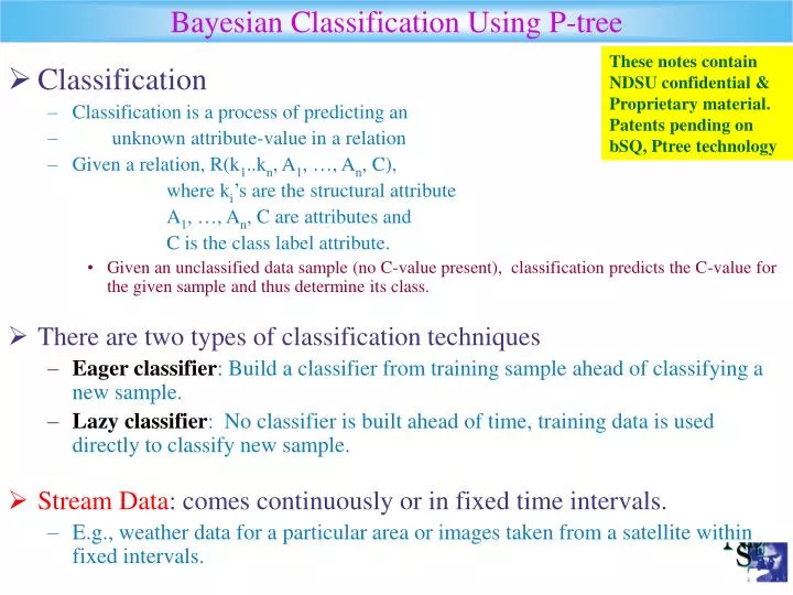
Bayesian Classification Using P-tree These notes contain NDSU confidential & Proprietary material. Patents pending on bSQ, Ptree technology • Classification • Classification is a process of predicting an • unknown attribute-value in a relation • Given a relation, R(k1..kn, A1, …, An, C), where ki’s are the structural attribute A1, …, An, C are attributes and C is the class label attribute. • Given an unclassified data sample (no C-value present), classification predicts the C-value for the given sample and thus determine its class. • There are two types of classification techniques • Eager classifier: Build a classifier from training sample ahead of classifying a new sample. • Lazy classifier: No classifier is built ahead of time, training data is used directly to classify new sample. • Stream Data: comes continuously or in fixed time intervals. • E.g., weather data for a particular area or images taken from a satellite within fixed intervals.
Preparing the data for Classification • Data Cleaning • Involves the handling of noisy data and missing values. • Noise could be removed or reduce by applying "smoothing" and missing values could be replaced with most common or some statistically determined value. • Relevance Analysis • In the given data not all its attributes are relevant to the classification task. • To reduce the task of classification these attribute should be identified and remove from classification task. • Data transformation • Data can be generalized using a concept hierarchy from low level to high level. • For spatial data, values of different bands are continuous numerical values. • We may intervalize them as high, medium, low etc. using the concept hierarchy.
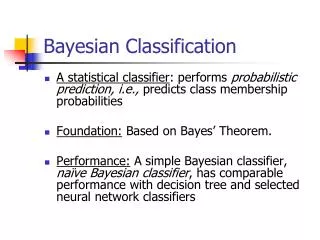
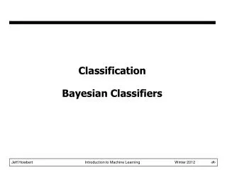
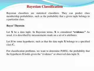
Bayesian Classification A Bayesian classifier is a statistical classifier, which is based on following theorem known as Bayes theorem: Bayes theorem: Let X be a data sample whose class label is unknown. Let H be a hypothesis (i.e., X belongs to class, C). P(H|X) is the posterior probability of H given X. P(H) is the probability of H, then P(H|X) = P(X|H)P(H)/P(X) Where P(X|H) is the posterior probability of X given H and P(X) is the probability of X.
Naïve Bayesian Classification • Given a relation R(K, A1..An, C) where K is the structure attribute and Ai and C are feature attributes. Also C is the class label attribute. • Each data sample is represented by feature vector, X=(x1..,xn) depicting the measurements made on the sample from A1,..An, respectively. • Given classes, C1,...Cm, the naive Bayesian Classifier will predict the class of unknown data sample, X, to be class, Cj having the highest posterior probability, conditioned on X • P(Cj|X) > P(Ci|X), where i j. (called the maximum posteriori hypothesis), • From the Bayes theorem: P(Cj|X) = P(X|Cj)P(Cj)/P(X) • P(X) is constant for all classes so we maximize P(X|Cj)P(Cj). If we assume equal likelihood of classes, maximize P(X|Cj) otherwise we maximize the whole product. • To reduce the computational complexity of calculating all P(X|Cj)'s the naive assumption of class conditional independence of values is used.
Naïve Bayesian Classification Class Conditional Independence: • This assumption says that the values of the attributes are conditionally independent of one another. So, P(X|Cj)=P(X1|Cj)*..*P(Xn|Cj). • Now the P(Xi|Cj)’s can be calculated directly from data sample. Calculating P(Xi|Cj) from P-trees: P(Xi|Cj) = sjxi/sj where sj = # of samples in class Cj and sjxi = # of training samples of class Cj, having Ai-value xi. These values can be calculated by: sjxi = RootCount [ (Pi(xi) ^ (PC(Cj) ], sj= RootCount [ PC(Cj)]
Non-Naive Bayesian Classifier (Cont.) • One problem with Non-Naïve-Bayesian P-tree classifiers: If the rc(Ptree(X))=0 then we will not get a class label for that tuple. • It could happen if the whole tuple is not present in the training data X1 X2 … Xk-1 Xk Xk+1 … Xn Whole tuple • Solution (Partial Naïve): So in that case we can divide the whole tuple into two parts separating one attribute from the whole tuple. e.g. Whole tuple X1 X2 … Xk-1 Xk Xk+1 … Xn X1 X2 … Xk-1 Xk+1 … Xn Xk Separated tuple X’ P(X|Ci)=rc[Ptree(X’) ^ PC(Ci)] * rc[Pk(Xk) ^ PC(Ci)] • Now the problem is how to select the attribute Xk • One way to use the information gain theory. • Calculate the info gain of all the attributes Xi then Xk is the one having lowest information gain
Information Gain Let C have m different classes, C1 to Cm The information needed to classify a given sample is: I(s1..sm) = -(i =1..m)[pi*log2(pi)] where pi=si/s is the probability that a sample belongs to Ci. A, an attrib, having values, {a1...av}. The entropy of A is E(A) = (j=1..v i=1..m sij/ s ) * I(s1j..smj) I(s1j..smj) = -i=1..m pij*log2(pij) where pij=sij/Sj is the probability that a sample in Ci belongs to Ai Information gain of A: Gain(A) = I(s1..sm) - E(A) si = rc(PC(ci) Sj = rc(PA(aj) sij = rc( PC(ci) ^ PA(aj) )
Performance of Ptree AND operation Bits NBC BCIG Performance of Classification:Comparison Performance for 4 classification classes Succ Succ IG Use 2 .14 .48 .40 3 .19 .50 .34 4 .27 .51 .32 5 .26 .52 .31 6 .24 .51 .27 7 .23 .51 .20 Performance of Classification:Classification success rate comparisons IG Use - Proportion of the number of times the information gain was used for successful classification.
Performance in Data Stream Application • Data Stream mining should have the following criteria • It must require a small constant time per record. • It must use only a fixed amount of main memory • It must be able to build a model at most one scan of the data • It must make a usable model available at any point of time. • It should produce a model that is equivalent to the one that would be obtained by the corresponding database-mining algorithm. • When the data-generating phenomenon is changing over time, the model at any time should be up-to-date but also include the past information. • Data Stream mining Using P-tree • It must require a small constant time per record. • P-tree require small and constant time. • It must use only a fixed amount of main memory • Ok for P-tree • It must be able to build a model at most one scan of the data • To build the P-tree only one scan is required • It must make a usable model available at any point of time. • Ok for P-tree • It should produce a model that is equivalent to the one that would be obtained by the corresponding database-mining algorithm. • Any conventional algorithm is also implementable with P-tree • When the data-generating phenomenon is changing over time, the model at any time should be up-to-date but also include the past information. • Ok for P-tree