Download
1 / 35
350 likes | 476 Views
In this talk, Michael Isard from Microsoft Research will present Dryad, a robust execution engine designed for batch processing of immutable datasets on commodity clusters. Dryad facilitates transparent scaling, efficient fault tolerance, and resource virtualization, enabling complex workloads beyond conventional SQL and HPC applications. Attendees will learn about DryadLINQ's programming model, the DAG abstraction for task scheduling, and real-world applications like data mining, graph algorithms, and K-means clustering across massive datasets, making it suitable for operations demanding significant computational resources.

E N D
Distributed computingusing Dryad Michael Isard Microsoft Research Silicon Valley
Distributed Data-Parallel Computing • Cloud • Transparent scaling • Resource virtualization • Commodity clusters • Fault tolerance with good performance • Workloads beyond standard SQL, HPC • Data-mining, graph analysis, … • Semi-structured/unstructured data
Execution layer • This talk: system-level middleware • Yuan Yu will describe DryadLINQ programming model on Saturday • Algorithm -> execution plan by magic
Problem domain • Large inputs • Tens of GB “small test dataset” • Single job up to hundreds of TB • Semi-structured data is common • Not latency sensitive • Overhead of seconds for trivial job • Large job could take days • Batch computation not online queries • Simplifies fault tolerance, caching, etc.
Talk overview • Some typical computations • DAG implementation choices • The Dryad execution engine • Comparison with MapReduce • Discussion
Map • Independent transformation of dataset • for each x in S, output x’ = f(x) • E.g. simple grep for word w • output line x only if x contains w
Map • Independent transformation of dataset • for each x in S, output x’ = f(x) • E.g. simple grep for word w • output line x only if x contains w S f S’
Map • Independent transformation of dataset • for each x in S, output x’ = f(x) • E.g. simple grep for word w • output line x only if x contains w S1 f S1’ S2 f S2’ S3 f S3’
Reduce • Grouping plus aggregation • 1) Group x in S according to key selector k(x) • 2) For each group g, output r(g) • E.g. simple word count • group by k(x) = x • for each group g output key (word) and count of g
Reduce • Grouping plus aggregation • 1) Group x in S according to key selector k(x) • 2) For each group g, output r(g) • E.g. simple word count • group by k(x) = x • for each group g output key (word) and count of g S G r S’
Reduce S G r S’
Reduce D is distribute, e.g. by hash or range S1 D G r S1’ S2 D G r S2’ S3 D G r S3’
Reduce ir is initial reduce, e.g. compute a partial sum S1 G ir D G r S1’ S2 G ir D G r S2’ S3 G ir D
K-means • Set of points P, initial set of cluster centres C • Iterate until convergence: • For each c in C • Initialize countc, centrec to 0 • For each p in P • Find c in C that minimizes dist(p,c) • Update: countc += 1, centrec += p • For each c in C • Replace c <- centrec/countc
K-means C0 ac cc C1 P ac cc C2 ac cc C3
K-means C0 ac cc C1 ac ac P1 P2 ac cc C2 P3 ac ac ac cc C3 ac ac
Graph algorithms • Set N of nodes with data (n,x) • Set E of directed edges (n,m) • Iterate until convergence: • For each node (n,x) in N • For each outgoing edge n->m in E, nm = f(x,n,m) • For each node (m,x) in N • Find set of incoming updates im = {nm: n->m in E} • Replace (m,x) <- (m,r(im)) • E.g. power iteration (PageRank)
PageRank N0 ae de N1 E ae de N2 ae de N3
PageRank cc N01 ae D N11 cc ae D N12 N02 ae D cc N13 N03 cc E1 ae D N21 cc ae D N22 E2 ae D cc N23 E3 cc ae D N31 cc ae D N32 ae D cc N33
DAG abstraction • Absence of cycles • Allows re-execution for fault-tolerance • Simplifies scheduling: no deadlock • Cycles can often be replaced by unrolling • Unsuitable for fine-grain inner loops • Very popular • Databases, functional languages, …
Rewrite graph at runtime • Loop unrolling with convergence tests • Adapt partitioning scheme at run time • Choose #partitions based on runtime data volume • Broadcast Join vs. Hash Join, etc. • Adaptive aggregation and distribution trees • Based on data skew and network topology • Load balancing • Data/processing skew (cf work-stealing)
Push vs Pull • Databases typically ‘pull’ using iterator model • Avoids buffering • Can prevent unnecessary computation • But DAG must be fully materialized • Complicates rewriting • Prevents resource virtualization in shared cluster S1 D G r S1’ S2 D G r S2’
Fault tolerance • Buffer data in (some) edges • Re-execute on failure using buffered data • Speculatively re-execute for stragglers • ‘Push’ model makes this very simple
Dryad • General-purpose execution engine • Batch processing on immutable datasets • Well-tested on large clusters • Automatically handles • Fault tolerance • Distribution of code and intermediate data • Scheduling of work to resources
Dryad System Architecture Scheduler R
Dryad System Architecture Scheduler R R
Dryad System Architecture Scheduler R R
Dryad Job Model • Directed acyclic graph (DAG) • Clean abstraction • Hides cluster services • Clients manipulate graphs • Flexible and expressive • General-purpose programs • Complicated execution plans
Dryad Inputs and Outputs • Partitioned data set • Records do not cross partition boundaries • Data on compute machines: NTFS, SQLServer, … • Optional semantics • Hash-partition, range-partition, sorted, etc. • Loading external data • Partitioning “automatic” • File system chooses sensible partition sizes • Or known partitioning from user
Channel abstraction S1 G ir D G r S1’ S2 G ir D G r S2’ S3 G ir D
Push vs Pull • Channel types define connected component • Shared-memory or TCP must be gang-scheduled • Pull within gang, push between gangs
MapReduce (Hadoop) • MapReduce restricts • Topology of DAG • Semantics of function in compute vertex • Sequence of instances for non-trivial tasks S1 f G ir D G r S1’ S2 f G ir D G r S2’ S3 f G ir D
MapReduce complexity • Simple to describe MapReduce system • Can be hard to map algorithm to framework • cf k-means: combine C+P, broadcast C, iterate, … • HIVE, PigLatin etc. mitigate programming issues • Implementation not uniform • Different fault-tolerance for mappers, reducers • Add more special cases for performance • Hadoop introducing TCP channels, pipelines, … • Dryad has same state machine everywhere
Discussion • DAG abstraction supports many computations • Can be targeted by high-level languages! • Run-time rewriting extends applicability • DAG-structured jobs scale to large clusters • Over 10k computers in large Dryad clusters • Transient failures common, disk failures daily • Trade off fault-tolerance against performance • Buffer vs TCP, still manual choice in Dryad system • Also external vs in-memory working set
Conclusion • Dryad well-tested, scalable • Daily use supporting Bing for over 3 years • Applicable to large number of computations • 250 computer cluster at MSR SVC, Mar->Nov 09 • 47 distinct users (~50 lab members + interns) • 15k jobs (tens of millions of processes executed) • Hundreds of distinct programs • Network trace analysis, privacy-preserving inference, light-transport simulation, decision-tree training, deep belief network training, image feature extraction, …