Download
1 / 12
120 likes | 233 Views
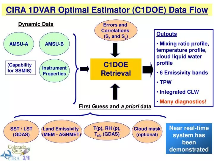
CIRA 1DVAR Optimal Estimator (C1DOE) Data Flow. Dynamic Data. Errors and Correlations (S a and S y ). Outputs Mixing ratio profile, temperature profile, cloud liquid water profile 6 Emissivity bands TPW Integrated CLW Many diagnostics!. AMSU-A. AMSU-B. Instrument Properties.

E N D
CIRA 1DVAR Optimal Estimator (C1DOE) Data Flow Dynamic Data Errors and Correlations (Sa and Sy) • Outputs • Mixing ratio profile, temperature profile, cloud liquid water profile • 6 Emissivity bands • TPW • Integrated CLW • Many diagnostics! AMSU-A AMSU-B Instrument Properties C1DOE Retrieval (Capability for SSMIS) First Guess and a priori data SST / LST (GDAS) Land Emissivity (MEM - AGRMET) Cloud mask (optional) T(p), RH (p), Tsfc (GDAS) Near real-time system has been demonstrated
Model Bias for 26 vertical RTM levels Minus 7 Levels CH 1 = 23.8 CH 2 = 31.4 CH 3 = 50.3 CH 4-8 = T(p) CH 16 = 89 CH 17 = 150 CH 18-20 = 183 4 4 2 2 26 level – 7 level RTM DTb Obs – Model (K) 0 0 window -2 -2 window windows windows -4 -4 1 2 3 4 5 6 7 8 16 17 18 19 20 1 2 3 4 5 6 7 8 16 17 18 19 20 Channel Channel Bias Correction for RTM Vital All zenith angles • Simulated TB’s calculated from pristine, clear sky, island sonde matchups and compared to AMSU TB’s. • Further refinement in progress
First guess atmosphere and surface Calculate weighting functions (sensitivity) Forward problem solved to yield estimates of the radiance in each channel Millimeter Wave Propagation (MPM92) Model (Liebe et al. 1993) Rayleigh cloud droplet absorption (Liebe et al. 1991) assuming a plane parallel, non-scattering atmosphere Match observed and modeled radiances Iterative process C1DOE Retrieval Methodology Additional details in Rodgers (2000)
Satellites provide measurements of radiation (i.e. brightness temperatures). The user must make use of models in order to extrapolate atmospheric parameters from these measurements. This is known as an inverse problem. The nature of inverse problems can be understood using the “footprint” analogy. Inverse problems
The relationship between the measured radiances, and the state vector is given by: where x is the state vector, b contains the model parameters, y is the measurement error, and f is the forward model. Inverse problems (cont.)
Linearizing about the real state vector and the real model parameters leads to: where x contains the estimated water vapor profiles, temperature profiles and 5 emissivities, and b is the estimated model parameter vector. The derivative terms are important for determining sensitivities of the radiances to both the model parameters and the water vapor profiles. Inverse problems (cont.)
OE is a method used to introduce constraints to a system A cost function must be minimized in order to find the optimal solution for the atmospheric state Optimal estimation
The cost function used in the C1DOE is given by: The first term is a penalty for deviating from the first guess (first guess and a priori are equivalent in this retrieval). This limits the outcome to only physical solutions. The second term is a penalty for deviations of the simulated radiances from the forward model output. This is a way to constrain the forward model and observational errors. Cost function
C1DOE cost function (Φ): Minimize Differences between Observed and Simulated Tbs Minimize Differences between a priori and retrieved states • *Error per channel (<= 3.5 K) • NEDT (noise) • Forward Model error • Biases: sensor - model • *A priori errors • q(p): 25-50% RH • w(p): 0.15 mm • T(p): 1.5 K, ε: 0.01 A priori ensures solution is physical and acts as a virtual measurement to further constrain the problem.
Data – The Advanced Microwave Sounding Unit (AMSU) • Two modules: AMSU – A and AMSU – B (MHS) • 20 channels: 23.8 to 183 GHz • Spatial resolution from 16 – 48 km at nadir • NEDT values ranging from 0.11 to 1.06 K (very low) • On NOAA satellites and Aqua Microwave Transmittance Spectrum 183 GHz used for moisture sounding
Data came from the Advanced Microwave Sounding Unit (AMSU) 20 channel microwave radiometer Ch. 1-15 used for temperature (AMSU-A) Ch. 16-20 used for water vapor (AMSU-B) AMSU
Table 3.3.2.1-1. Channel Characteristics and Specifications of AMSU-A AMSU-A Channelization