Download
1 / 22
230 likes | 259 Views
Explore WCS keywords in FITS files and common AIPS tasks. Learn about XMM calibration, hardness ratios, and photon index vs. energy index. Discover key elements like CRVAL, CRPIX, and more in WCS. Uncover essential AIPS tasks like FITLD and IMAGR for data calibration. Dive into XMM Calibration quantities and exposure relations for efficient data analysis.

E N D
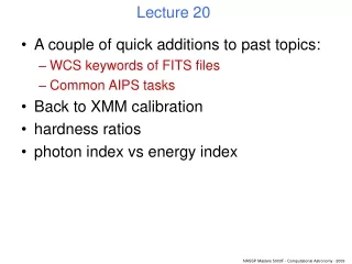
Lecture 20 • A couple of quick additions to past topics: • WCS keywords of FITS files • Common AIPS tasks • Back to XMM calibration • hardness ratios • photon index vs energy index
WCS keywords of FITS files • WCS stands for World Coordinate System. • http://fits.gsfc.nasa.gov/fits_wcs.html • What they’re for: pixellated data – ie samples of some quantity on a regular grid. • WCS keywords define the mapping between the pixel index and a world coordinate system. • Eg: a 2d image of the sky. We want to know which sky direction the (j,k)th pixel corresponds to.
Eg, projection onto a tangent plane. WCS must encode the relation between θ and the pixel number. Pixel grid on tangent plane θ
WCS example continued w- wref The general formula in this case is (p - pref) * scale = tan(w – wref). p is the pixel coordinate and w the world coordinate. w might eg be right ascension or declination. p- pref • WCS must describe 4 things: • pref • wref • scale • the nature of the functional relation. • Perhaps also world units. Note: (1) pref can be real-valued; (2) By convention, p at the centre of the 1st pixel = 1.0.
WCS keywords for array extensions • In what follows, n is an integer, corresponding to one of the dimensions of the array. • CRVALn – wref. • CRPIXn – pref. • CDELTn – scale. • CTYPEn – an 8-character string encoding the function type (eg ‘TAN---RA’). There is an agreed list of these. • CUNITn – string encoding the unit of w (eg ‘deg’). Also an agreed list. • In addition, rotated coordinate systems can be defined via either addingPCi_j keywords to the above scheme, or replacing CDELTn by CDi_j keywords. But I don’t want to get too deeply into this. • Analogous (starting with T) WCS keywords are also defined for table columns.
Now... a little word more about AIPS. • If you look at the cookbook, you will see there are hundreds of AIPS tasks. It is a bit daunting. • However, you will probably only ever use the following: • FITLD – to import your data from FITS. • IBLED – lets you flag bad data. • CALIB – to calculate calibration tables. • SPLIT – splits your starting single observation file into 1 UV dataset per source. • Usually you will observe 3 or maybe 4 sources during your observation – the target, a primary and secondary flux calibrator and a phase calibrator. • IMAGR – to calibrate, grid, FT and clean your data. • FITAB – exports back to FITS.
Back to XMM.Calibration quantities: (1) Quantum Efficiency Silicon K edge Oxygen K edge
(2) Effective area (no filter) (includes QE) Gold M edge
Effective Area change with filters This is for pn – MOS is very similar.
Exposure • Relation between incident flux density S and the photon flux density φ: most general form is where A is an effective area and the fractional exposure kernel X contains all the information about how the photon properties are attenuated and distributed. • Note I didn’t include a t' because in XMM there is no redistribution (ie ‘smearing’) mechanism which acts on the arrival time. • Vector r is shorthand for x,y. dimensionless erg s-1 eV-1 cm-2 cm2 photons s-1 eV-1 E of course is the photon energy.
Exposure • A reasonable breakdown of AX is where • R is the redistribution matrix; • A is the on-axis effective area (including filter and QE contributions); • V is the vignetting function; • C holds information about chip gaps and bad pixels; • ρ is the PSF (including OOTE and RGA smearing); and • D is a ‘dead time’ fraction, which is a product of • a fixed fraction due to the readout cycle, and • a time-variable fraction due to blockage by discarded cosmic rays. • the fraction of ‘good time’ during the observation. All dimensionless except A.
Exposure • This includes a number of assumptions, eg • The spacecraft attitude is steady. • Variations between event patterns are ignored. • No pileup, etc etc • Now we try to simplify matters. First, let’s only consider point sources, ie This gets rid of the integral over r, and the r‘ in V and ρ become r0.
Exposure • What we do next depends on the sort of product which we want. There are really only 4 types (XMM pipeline products) to consider:
Exposure map • For XMM images we have where the exposure mapε is and the energy conversion factor (ECF) ψ is calculated by integrating over a model spectrum times R times A. • Hmm well, it’s kind of roughly right. photons cm2 eV s-1 erg-1 photons erg s-1 eV-1 cm-2 s
ARF • For XMM spectra where the ancillary response function (ARF) α is This is a bit more rigorous because the resulting spectrum q is explicitly acknowledged to be pre-RM. • And if S can be taken to be time-invariant, then this expression follows almost exactly from the general expression involving X. photons eV-1
Fractional exposure • For XMM light curves, where the fractional exposuref is photons s-1
Sources • There is just a small modification to the ‘image’ approximation: This is probably the least rigorous of the three product-specific distillations of X. • To some extent, this idiosyncratic way of cutting up the quantities is just ‘what the high-energy guys are used to’.
Prescriptions to obtain ergs s-1: • Image: • Divide by exposure map • Multiply by ECF • Spectrum: • You don’t. Compare to forward-treated model instead. • Light curve: • Divide by frac exp • Multiply by ECF • Source: • As for image but also divide by integral of ρC.
Some spectral lore: (1) Hardness ratios. • This is a term you will encounter often in the high-energy world. • Add up the counts within energy band 1 C1; • add up the counts in band 2 C2; • the hardness ratio is defined as • Clearly confined to the interval [-1,1]. • It is a crude but ready measure of the spectral properties of the source. • Uncertainties are often tricky to calculate.
Some spectral lore: (2) Photon index. • Suppose a source has a power spectrum, ie • As we know, α is called the spectral index. If we plot log(S) against log(E), we get a straight line of slope α. • But! Think how we measure a spectrum. We have to count photons and construct a frequency histogram – so many within energy bin foo, etc.
Photon frequency histogram Total energy S of all the N photons in a bin of centre energy E is (about) N times E. Photon energy
Photon index. • Thus the energy spectrum S(E) and the photon spectrum N(E) are related by • Hence, if then • photon index is always 1 less than the spectral index. Matters aren’t helped by the habit to use eV for the photon energy but ergs for the total energy!