Download

1 / 30
300 likes | 536 Views
Evolution strategies. Chapter 4. ES quick overview. Developed: Germany in the 1970’s Early names: I. Rechenberg, H.-P. Schwefel Typically applied to: numerical optimisation Attributed features: fast good optimizer for real-valued optimisation relatively much theory Special:

E N D
Evolution strategies Chapter 4
ES quick overview • Developed: Germany in the 1970’s • Early names: I. Rechenberg, H.-P. Schwefel • Typically applied to: • numerical optimisation • Attributed features: • fast • good optimizer for real-valued optimisation • relatively much theory • Special: • self-adaptation of (mutation) parameters standard
Introductory example • Task: minimimise f : Rn R • Algorithm: “two-membered ES” using • Vectors from Rn directly as chromosomes • Population size 1 • Only mutation creating one child • Greedy selection
Introductory example: pseudocde • Set t = 0 • Create initial point xt = x1t,…,xnt • REPEAT UNTIL (TERMIN.COND satisfied) DO • Draw zi from a normal distr. for all i = 1,…,n • yit = xit + zi • IF f(xt) < f(yt) THEN xt+1 = xt • ELSE xt+1 = yt • FI • Set t = t+1 • OD
Introductory example: mutation mechanism • z values drawn from normal distribution N(,) • mean is set to 0 • variation is called mutation step size • is varied on the fly by the “1/5 success rule”: • This rule resets after every k iterations by • = / c if ps > 1/5 • = • c if ps < 1/5 • = if ps = 1/5 • where ps is the % of successful mutations, 0.8 c 1
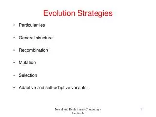
Representation • Chromosomes consist of three parts: • Object variables: x1,…,xn • Strategy parameters: • Mutation step sizes: 1,…,n • Rotation angles: 1,…, n • Not every component is always present • Full size: x1,…,xn,1,…,n,1,…, k where k = n(n-1)/2 (no. of i,j pairs)
Mutation • Main mechanism: changing value by adding random noise drawn from normal distribution • x’i = xi + N(0,) • Key idea: • is part of the chromosome x1,…,xn, • is also mutated into ’ (see later how) • Thus: mutation step size is coevolving with the solution x
Mutate first • Net mutation effect: x, x’, ’ • Order is important: • first ’ (see later how) • then x x’ = x + N(0,’) • Rationale: new x’ ,’ is evaluated twice • Primary: x’ is good if f(x’) is good • Secondary: ’ is good if the x’ it created is good • Step-size only survives through “hitch-hiking” • Reversing mutation order this would not work
Mutation case 1:Uncorrelated mutation with one • Chromosomes: x1,…,xn, • ’ = • exp( • N(0,1)) • x’i = xi + ’• N(0,1) • Typically the “learning rate” 1/ n½ • And we have a boundary rule ’ < 0 ’ = 0
Mutants with equal likelihood Circle: mutants having the same chance to be created
Mutation case 2:Uncorrelated mutation with n ’s • Chromosomes: x1,…,xn, 1,…, n • ’i = i• exp(’ • N(0,1) + • Ni (0,1)) • x’i = xi + ’i• Ni (0,1) • Two learning rate parameters: • ’ overall learning rate • coordinate wise learning rate • 1/(2 n)½ and 1/(2 n½) ½ • Boundary rule: i’ < 0 i’ = 0
Mutants with equal likelihood Ellipse: mutants having the same chance to be created
Mutation case 3:Correlated mutations • Chromosomes: x1,…,xn, 1,…, n ,1,…, k where k = n • (n-1)/2 • Covariance matrix C is defined as: • cii = i2 • cij = 0 if i and j are not correlated • cij = ½•(i2 - j2 ) •tan(2 ij) if i and j are correlated • Note the numbering / indices of the ‘s
Correlated mutations cont’d The mutation mechanism is then: • ’i = i•exp(’ • N(0,1) + • Ni (0,1)) • ’j = j + • N (0,1) • x ’ = x + N(0,C’) • x stands for the vector x1,…,xn • C’ is the covariance matrix C after mutation of the values • 1/(2 n)½ and 1/(2 n½) ½ and 5° • i’ < 0 i’ = 0 and • | ’j | > ’j =’j- 2 sign(’j) • NB Covariance Matrix Adaptation Evolution Strategy (CMA-ES) isprobably the best EA for numerical optimisation, cf. CEC-2005 competition
Mutants with equal likelihood Ellipse: mutants having the same chance to be created
Recombination • Creates one child • Acts per variable / position by either • Averaging parental values, or • Selecting one of the parental values • From two or more parents by either: • Using two selected parents to make a child • Selecting two parents for each position anew
Parent selection • Parents are selected by uniform random distribution whenever an operator needs one/some • Thus: ES parent selection is unbiased - every individual has the same probability to be selected • Note that in ES “parent” means a population member (in GA’s: a population member selected to undergo variation)
Survivor selection • Applied after creating children from the parents by mutation and recombination • Deterministically chops off the “bad stuff” • Two major variants, distinguished by the basis of selection: • (,)-selection based on the set of children only • (+)-selection based on the set of parents and children:
Survivor selection cont’d • (+)-selection is an elitist strategy • (,)-selection can “forget” • Often (,)-selection is preferred for: • Better in leaving local optima • Better in following moving optima • Using the + strategy bad values can survive in x, too long if their host x is very fit • Selective pressure in ES is high compared with GAs, • 7 • is a traditionally good setting (decreasing over the last couple of years, 3 • seems more popular lately)
Self-adaptation illustrated • Given a dynamically changing fitness landscape (optimum location shifted every 200 generations) • Self-adaptive ES is able to • follow the optimum and • adjust the mutation step size after every shift !
Prerequisites for self-adaptation • > 1 to carry different strategies • > to generate offspring surplus • Not “too” strong selection, e.g., 7 • • (,)-selection to get rid of misadapted ‘s • Mixing strategy parameters by (intermediary) recombination on them
Example application: the cherry brandy experiment • Task: to create a colour mix yielding a target colour (that of a well known cherry brandy) • Ingredients: water + red, yellow, blue dye • Representation: w, r, y ,b no self-adaptation! • Values scaled to give a predefined total volume (30 ml) • Mutation: lo / med / hi values used with equal chance • Selection: (1,8) strategy
Example application: cherry brandy experiment cont’d • Fitness: students effectively making the mix and comparing it with target colour • Termination criterion: student satisfied with mixed colour • Solution is found mostly within 20 generations • Accuracy is very good
Example application: the Ackley function (Bäck et al ’93) • The Ackley function (here used with n =30): • Evolution strategy: • Representation: • -30 < xi < 30 (coincidence of 30’s!) • 30 step sizes • (30,200) selection • Termination : after 200000 fitness evaluations • Results: average best solution is 7.48 • 10 –8 (very good)