Download
1 / 31
310 likes | 374 Views
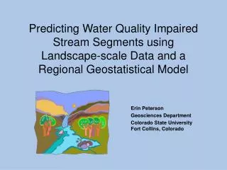
Regional GIS-based Geostatistical Models for Stream Networks. Erin E. Peterson Postdoctoral Research Fellow CSIRO Mathematical and Information Sciences Division Brisbane, Australia May 18, 2006. This research is funded by. This research is funded by. U.S.EPA. U.S.EPA. 凡.

E N D
Regional GIS-based Geostatistical Models for Stream Networks Erin E. Peterson Postdoctoral Research Fellow CSIRO Mathematical and Information Sciences Division Brisbane, Australia May 18, 2006
This research is funded by This research is funded by U.S.EPA U.S.EPA 凡 Science To Achieve Science To Achieve Results (STAR) Program Results (STAR) Program Cooperative Cooperative CR CR - - 829095 829095 # # Agreement Agreement Space-Time Aquatic Resources Modeling and Analysis Program The work reported here was developed under STAR Research Assistance Agreement CR-829095 awarded by the U.S. Environmental Protection Agency (EPA) to Colorado State University. This presentation has not been formally reviewed by EPA. EPA does not endorse any products or commercial services mentioned in this presentation.
Collaborators Dr. David M. Theobald Natural Resource Ecology Lab Department of Recreation & Tourism Colorado State University, USA Dr. N. Scott Urquhart Department of Statistics Colorado State University, USA Dr. Jay M. Ver Hoef National Marine Mammal Laboratory, Seattle, USA Andrew A. Merton Department of Statistics Colorado State University, USA
Overview Introduction ~ Background ~ Develop and compare geostatistical models ~ Visualizing model predictions ~ Current and future research in SEQ
Challenges • Challenges are similar to states attempting to comply with the Clean Water Act • Anadromous Waters Catalog (AWC) • Large number of water bodies within AK • ~ 20,000 unidentified anadromous water bodies • Need spatially explicit, unambiguous field observations of anadromous fish • Cost (time and $$) of field surveys is high • “… We recognize a pressing need for approaches that predict the distribution of salmon in Alaska’s extensive unsurveyed freshwaters.”
My Goal • Demonstrate a geostatistical methodology based on • Coarse-scale GIS data • Field surveys • Predict stream characteristics for individual segments throughout a region
How are geostatistical models different from traditional statistical models? • Traditional statistical models (non-spatial) • Residual error (ε) is assumed to be uncorrelated • ε = unexplained variability in the data • Geostatistical models • Residual errors are correlated through space • Spatial patterns in residual error resulting from unidentified process(es) • Model spatial structure in the residual error • Explain additional variability in the data • Generate predictions at unobserved sites
10 Sill Semivariance Nugget Range 0 1000 0 Separation Distance Geostatistical Modeling • Fit an autocovariance function to data • Describes relationship between observations based on separation distance • 3 Autocovariance Parameters • Nugget: variation between sites as separation distance approaches zero • Sill: delineated where semivariance asymptotes • Range: distance within which spatial autocorrelation occurs
B A C Distance Measures and Spatial Relationships • Straight Line Distance (SLD) • As the crow flies
B A C Distance Measures and Spatial Relationships • Symmetric Hydrologic Distance (SHD) • As the fish swims
B A C Distance Measures and Spatial Relationships • Weighted asymmetric hydrologic distance (WAHD) • As the water flows • Incorporate flow direction & flow volume Ver Hoef, J.M., Peterson, E.E., and Theobald, D.M. (2006) Spatial Statistical Models that Use Flow and Stream Distance, Environmental and Ecological Statistics, to appear.
Distance Measures and Spatial Relationships • Fit a mixture of covariances B A C • Based on more than one distance measure Cressie, N., Frey, J., Harch, B., and Smith, M.: 2006, ‘Spatial Prediction on a River Network’, Journal of Agricultural, Biological, and Environmental Statistics, to appear.
Distance measure influences how spatial relationships are represented in a stream network • Site’s relative influence on other sites • Dictates form and size of spatial neighborhood • Important because… • Impacts accuracy of the geostatistical model predictions SHD WAHD SLD Distance Measures and Spatial Relationships
Dissolved Organic Carbon (DOC) Example Demonstrate how a geostatistical methodology can be used to identify ecologically significant waters Example: • Develop and compare geostatistical models for DOC • Predict regional DOC levels • Identify the spatial location of stream segments with high levels of DOC
2 1 3 1 2 3 1 2 3 SHD AHD SLD Functional Linkage of Watersheds and Streams (FLoWS) • Create data for geostatistical modeling • Calculate watershed covariates for each stream segment • Calculate separation distances between sites • SLD, Asymmetric hydrologic distance (AHD) • Calculate the spatial weights for the WAHD • Convert GIS data to a format compatible with statistics software • FLoWS website: http://www.nrel.colostate.edu/projects/starmap
Watershed Segment B Watershed Segment A • Calculate the PI of each upstream segment on segment directly downstream A B • Calculate the PI of one survey site on another site • Flow-connected sites • Multiply the segment PIs C Watershed Area A Segment PI of A = Watershed Area A+B Spatial Weights for WAHD • Proportional influence (PI):influence of each neighboring survey site on a downstream survey site • Weighted by catchment area: Surrogate for flow volume
Calculate the PI of each upstream segment on segment directly downstream A C B E D • Calculate the PI of one survey site on another site • Flow-connected sites • Multiply the segment PIs F G H Spatial Weights for WAHD • Proportional influence (PI):influence of each neighboring survey site on a downstream survey site • Weighted by catchment area: Surrogate for flow volume survey sites stream segment
Calculate the PI of each upstream segment on segment directly downstream • Calculate the PI of one survey site on another site • Flow-connected sites • Multiply the segment PIs Site PI = B * D * F * G Spatial Weights for WAHD • Proportional influence (PI):influence of each neighboring survey site on a downstream survey site • Weighted by catchment area: Surrogate for flow volume A C B E D F G H
Data for Geostatistical Modeling • Distance matrices • SLD, AHD • Spatial weights matrix • Contains flow dependent weights for WAHD • Watershed covariates • Lumped watershed covariates • Mean elevation, % Urban • Observations • MBSS survey sites
Geostatistical Modeling Methods • Fit the correlation matrix for SLD and WAHD models Maximized profile-log likelihood function • Estimate model parameters • Comparison within model set • Spatial AICC • Comparison between model set • Universal kriging • MSPE
SLD Mariah Model r2 Observed vs. Predicted values • 1 influential site • r2 without site = 0.66
Squared Prediction Error (SPE) Spatial Patterns in Model Fit
Generate Model Predictions • Prediction sites • Study area • 1st, 2nd, and 3rd order non-tidal streams • 3083 segments = 5973 stream km • ID downstream node of each segment • Create prediction site • Generate predictions and prediction variances • SLD Mariah model • Universal kriging algorithm
Implications for Anadromous Fish Conservation • Apply this methodology to salmon or salmon habitat • Identify habitat conditions necessary for spawning, rearing, or migration of anadromous fish • Based on ecological & biological knowledge • Identify watershed conditions that may influence those conditions • Watershed geology type ~ substrate type • Derive watershed characteristics using GIS/remote sensing • Generate predictions and estimates of uncertainty for potential salmon habitat • Categorize predictions into low, medium, or high status • Probability of supporting anadromous fish
Implications for Anadromous Fish Conservation • Tradeoff between cost-efficiency and model accuracy • One model can be used throughout a large region • Regions may be ecologically unique • May need to generate separate models for AWC regions • Allocate scarce sampling resources efficiently • Target areas with a high probability of supporting anadromous fish • Identify areas where more information would be useful
Implications for Anadromous Fish Conservation Advantages of GIS • Identify spatial patterns in model fit • Evaluate habitat at multiple scales • Feature scale and regional scale • Help prioritize fish habitat restoration • Help prioritize land/conservation easement acquisitions • Easily communicate with community, environmental, and government groups
Questions? Comments? Erin E. Peterson Phone: +61 7 3214 2914 Email: Erin.Peterson@csiro.au