Download
1 / 36
470 likes | 1.17k Views
Real-Time Quantitative Reverse Transcription Polymerase Chain Reaction ( qRT -PCR) Analysis. Jelena Brkic BIOL5081. What is Real-Time qRT -PCR?. An in vitro method for enzymatically amplifying defined sequences of RNA

E N D
Real-Time Quantitative Reverse Transcription Polymerase Chain Reaction (qRT-PCR) Analysis Jelena BrkicBIOL5081
What is Real-Time qRT-PCR? • An in vitro method for enzymatically amplifying defined sequences of RNA • From all the available quantification techniques it has the highest sensitivity, reproducibility, simplicity and dynamic range • Variety of applications: • Relative expression of mRNAs • Validation of microarray data • Clinical Diagnostics
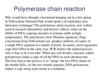
Real Time • signals (generally fluorescent) are monitored as they are generated and are tracked throughout the program • Quantitative • Quantitatively measures the amplification of template • Reverse Transcription • Refers to the reverse transcription of the RNA starting material into cDNA • This step can be conducted in a one-step or more traditionally two-step method • Polymerase Chain Reaction • Method dependent on thermo cycling and enzymes allowing for amplification of small starting material of DNA First generate cDNAthen perform PCR
Analyzing qRT-PCR Data • Two most commonly used methods to analyze data: • Absolute Quantification • Used for copy number determination, viral load etc. • Conducted by relating the PCR signal to a standard curve • Will give you absolute quantification that can be expressed in units • Relative Quantification • Gene expression studies • Measured against a calibrator sample and expressed as an n-fold difference relative to the calibrator • Often normalized to an internal control – housekeeping gene • Controls for loading artificats
qRT-PCR – The Basics • Isolate RNA from samples • Reverse Transcription • Pick Reference Gene • Design Primers • Run qRT-PCR • Fluorescent signal (eg. Taqman, SYBERGreen) • Acquire signal at end of each cycle • Analyze • Set Threshold • Obtain CT values
qRT-PCR – The Basics • qRT-PCR exploits the fact that the quantity of PCR products in exponential phase is in proportion to the quantity of initial template under ideal conditions • Threshold: an arbitrary level of fluorescence chosen on the basis of the baseline variability • Can be adjusted for each experiment so that it is in the region of exponential amplification across all plots • Ct: “Cross threshold” is a basic principle of real time PCR and is an essential component in producing accurate and reproducible data • Defined as the fractional PCR cycle number at which the reporter fluorescence is greater than the threshold Threshold CT Starting amount of template (?) Reaction Tubes
Understanding the Output… • PCR has three phases: • Exponential • Earliest segment in the PCR • Product increases exponentially • Reagents are not limited • Linear • Linear increase in product • PCR reagents become limited • Plateau • Later cycles of PCR • Reagents become depleted • Amplification not equal
The threshold for Ct determination should be set up as close as possible to the base of the exponential phase Picking the best CT value
Factors Affecting qRT-PCR Results • Normalization • Relative Quantification Methods • Amplification Efficiency • Power and Sample Size Specificity of primerscan easily be checked bygel electrophoresis
Normalization • Most commonly expression of target genes is normalized against an endogenous control (HKG) • KEY ASSUMPTION: the expression level of the gene remains constant across different experimental conditions. Therefore serves as a control for loading artifacts. • Selecting a HKG from literature may not always be the best choice – should be part of experimental protocol: • Gene Stability Parameter (M) • ANOVA
Methods for Housekeeping Gene selection • Gene-stability parameter (M): • The average pairwise variation of a particular gene with all other control genes • Genes with small M are considered to be most stable Genorm, Normfinder,Bestkeeper algorithms
Example: We want to assess the relative expression levels of gene X in mice ovaries after treatment of mice with different doses of hormone Y. First we must choose the best housekeeping gene to use in our relative quantification. Two housekeeping genes (HK001 and HK002) were selected for an experiment with 5 dose groups (A-E) with 5 animals (n=5) in each dose group. QRT-PCR was performed and CT values were obtained for both genes. a = number of treatments = 5 N = number of animals = 25
Analysis of Variance (ANOVA) – One way • Partition the variability in a set of data into component parts SSTotal = SSTreatment + SSError Total variance = Differences between groups due to treatment +Variances within groups due to “error”
Analysis of Variance (ANOVA) – One way • To make sources of variability comparable the sum of squares is divided by the respective degrees of freedom to obtain mean squares • The ratio of Mean Square yields the F statistic DFG = a-1 = 4 DFE = N-a = 20 DFT = N-1 = 24
Order of input: Animal, dose, gene notation and Ct value Continue in SAS… data table; input anim dose$ gene$ Ct; Cards; 1 A HK001 20.30 2 A HK001 20.57 data missing … 24 E HK002 20.10 25 E HK002 20.25 ; proc ANOVA; by gene; class dose; model Ct=dose; run; Cards = data immediately follows on next line Insert all data values in order specified abovefor all genes you are comparing Proc ANOVA for balanced design CLASS: Classification statementMODEL: Response = treatment levels
Continue in SAS… Box Plots of dose vs. Ct • HK001 more variable • Continue by looking at the F-statistic and P-value HK001 HK002
Continue in SAS… • F-statistic close to 1 = the two sources of variability are approximately equal • A HKG that remains constant across different conditions will have a small F-statistic compared to other genes • “Optimum HKG” is defined based on a non-significant(p>0.05), minimum F-statistic • If none of the genes yield a non-significant F-statistic then none is suitable to be used as a housekeeping gene.
Normalization gene selected Example: Mice were treated with or without Hormone Y for 10 days after which ovaries were removed and expression levels of TG001 and TG002 were measured along with HK002 as the reference gene. For each dose n=4, and each sample was performed in triplicate. Are the Ct values too high/low? How do the technical triplicates look?
Relative Quantification Methods: • ΔΔCT Method – Livak Method • KEY ASSUMPTION: Amplification efficiency is 2 for both the target and reference gene • This indicates a doubling of PCR product with each cycle (exponential growth) • Presented as a ratio: Ratio = 2-ΔΔCt
Ratio = 2-ΔΔCt Understanding the Ratio… • Where ΔΔCt = ΔCttreated – ΔCtcontrol • ΔCttreated= Ct difference of a reference and target gene for a treatment sample • ΔCttreated= Cttarget – Ctref • ΔCtcontrol= Ct difference of a reference and target gene for a control sample • ΔCtcontrol= Cttarget – Ctref Note: for a full derivation of the above equation refer to Ref 1.
Thinking about your experimental set-up… • Exactly how the averaging is performed depends on your experimental set up. • Biological replicates (separate RNA preparations) • Treat each sample separately • Average the results after the ratio is calculated • Technical replicates (PCR replicates) • More appropriate to average the Ct data before performing the ratio • Separate wells: • There is no reason to pair any particular target well with any particular reference well. • First we want to average the target and reference Ct values separately before performing the ΔCt calculation • Same well: • Same starting cDNA with the use of multiple dyes • Can calculate the ΔCt value for each well separately • The ΔCt values can be averaged before proceeding with the ratio
ΔΔCt = ΔCttreated – Δctcontrol Separate wells… • Calibrate our treatment to our control and find the ratio • 1st we average all of the target and reference Ct values • 2ndwe normalize our target Ct values to our internal control = AvgΔCt- AvgΔCtcalibrator= ΔΔCt = 2^-ΔΔCt =AVERAGE(Cell1:Cell12) = Avgtaget Ct- Avg ref Ct= 23.78 - 19.91 = 3.87
Check for variability in control… E2 E4 =AVERAGE(Cell1:Cell12) =2^(-((C2-D2)-($E$2-$E$4)))
Simple in Excel… =STDEV(Cells of Control) =STDEV/SQRT(12) Test the hypothesis: H0 : μc = μt Ha : μc ≠ μt T-test, ANOVA etc.
Efficiency Corrected Model – Pffafl Method • If the assumptions behind the ΔΔCT Method are not valid, the efficiency corrected model can be employed instead • Where: • ETARGET = target gene amplification efficiency • E REF = ref gene amplification efficiency • ΔCttarget= Ctcontrol– Cttreated diff. btw Ct of treated vs control for target gene • ΔCtref= Ctcontrol– Cttreated diff. btw Ct of treated vs control for ref gene • E is in the range from 1 (minimum) to 2 (theoretical maximum/optimum) • The “efficiency adjustment” is defined as EA=log2(efficiency) • The above equation can be re-written as:
Avg Control-Avg Treatment Efficiency Corrected Model • Sample Calculation: HK002 E=1.85, TG001 E=2 EA = log2(1.85) = 0.8875
Amplification Efficiency • In order to use the efficiency corrected model we need to be able to estimate the amplification efficiencies for all of our genes • Many ways of doing this… • Relative Standard Curve • Serial dilutions of all genes analyzed run with samples • Plotted as Ct vs. log10(cDNA input) • PCR efficiency calculated according to the relationship: E=10(-1/slope) • Fitting linear, sigmoidal or multiple models
Relative Standard Curve This is a very reproducible method however it often reports efficiencies greater than 2 which are not theoretically possible and implies an overestimation of the ‘real’ efficiency (Efficiencies range from 1.60- over 2)
Power and Sample Size • Power is dependent on sample size, significance criterion (α), effect size and sample standard deviation • Prospective sample size calculations are important in the planning of an experiment • Insufficient power may render any conclusions from an experiment as useless • Due to high variability of same samples in different laboratories the power calculation can be calculated after the effect and SD are observed from a pilot study
Calculate in SAS… • How many animals do we need per group to achieve power of 0.80, detect a group mean difference of 1.0 between treated and control Ct values? The SD ranges between 0.40-0.50. procpower; twosamplemeans meandiff=1 stddev = 0.400.450.50 power = 0.8 npergroup=.; run;
Conclusions • No housekeeping gene is perfect for all applications • Multiple housekeeping genes should be run for each experimental set up – varies by sample type, primer/probe combination, detection chemistry, tubes, real-time cycler platform • Relative quantification must be highly validated to generate useful and biologically relevant information • Careful think about the experimental set-up • Block effects? • RT Efficiencies? • PCR inhibitors in exogenous control set ups etc. • Many mathematical models exist, as well as software, choose carefully which model is best suited for your experimental set-up, question and limitations • Use of three biological replicates and at least two technical replicates is advised for greater validity • Reproducibility can be tested with the coefficient of variability for intra and inter-assay variation
SASqPCR: Robust and Rapid Analysis of RT-qPCR Data in SAS • An all-in-one computer program allowing users to perform RT-qPCR data analysis in a more flexible and convenient way • Developed using SAS software https://code.google.com/p/sasqpcr/downloads/list
Useful Resources and References • Livak, K. J. and T. D. Schmittgen (2001). "Analysis of relative gene expression data using real-time quantitative PCR and the 2(-Delta Delta C(T)) Method." Methods25(4): 402-408. • Khan-Malek, R. and Y. Wang (2011). "Statistical analysis of quantitative RT-PCR results." Methods Mol Biol691: 227-241. • Pfaffl, M. W. (2001). "A new mathematical model for relative quantification in real-time RT-PCR." Nucleic Acids Res29(9): e45. • Yuan, J. S., A. Reed, et al. (2006). "Statistical analysis of real-time PCR data." BMC Bioinformatics7: 85. • http://www.vetmed.ucdavis.edu/vme/taqmanservice/pdfs/qPCR_guidelines.pdf