Download
1 / 16
160 likes | 166 Views
HARRIS’s Ch. 10-12. Supplement Zumdahl’s Chapter 15. Harris Chapter 10 Buffer Capacity, Ionic Strength and Henderson – Hasselbalch Harris Chapter 11 Diprotics Intermediate form Buffers Fractional Composition. Harris Chapter 12 Titration accuracy limit Diprotic titration

E N D
HARRIS’s Ch. 10-12 Supplement Zumdahl’s Chapter 15
Harris Chapter 10 Buffer Capacity, Ionic Strength and Henderson–Hasselbalch Harris Chapter 11 Diprotics Intermediate form Buffers Fractional Composition Harris Chapter 12 Titration accuracy limit Diprotic titration Indicated indicators Spreadsheet Titration Curves Monoprotic Diprotic Triprotic Supplementary Content
Buffer Capacity, • Buffers resist pH change only while both forms present in significant quantity. • We want slope of pH with Cbase to be low! • Alternately, dCb/dpH should be high and represents , the capacity to resist. • = (ln 10) SA / (S+A) while H–H viable. • Limits: min=2.303 [smaller], max=1.152 [S=A]
Henderson–Hasselbalch • pH = pKa + log( aS / aA ) pKa + log([S]/[A]) • aY = Y [Y] = thermodynamic “activity” • Y = “activity coefficient,” a correction factor, well known for dilute ionic solutions. (Ch. 8) • For Yz±, ion of radius (pm) in a solution of many ions and = ½ ci zi2 is ionic strength, log Y = – 0.51z2½ / [ 1 + ( ½ / 305) ]
Diprotic Intermediate Form • H2A HA– + H+ (abbreviated below as A B + H) • HA– A2– + H+ (abbreviated below as B C + H) • HA– is the intermediate (amphiprotic) form. • HA– dominates at 1st equivalence point, where ~ zero! World’s worst buffer. • Also, near equivalence, Kw is important (to all conjugates), and must be included. How?
Explicit Water Equilibrium • If both H+and OH– are important, they must be included in MHA’s charge balance: • [H+] + [M+] = [HA–] + 2[A2–] + [OH–] or • H + F H + (A + B + C) = B + 2C + Kw/H • H = C – A + Kw/H = K2B/H – HB/K1 + Kw/H • H2 = K2B – H2B/K1 + Kw • H2 (B/K1 + 1) = K2B + Kw
Solution from B = HA– • H = [ (K1 K2 B + K1 Kw) / (B + K2) ] ½ • But if weak [B]0 = F, then Beq F >> K2 • H [ (K1 K2 F + K1 Kw) / F ] ½ • And if Kw << F K2 • H ~ [ K1 K2 F / F ] ½ = (K1 K2) ½ • pH ~ ½ (pK1 + pK2) • Like pH = pKa at V½ for monoprotic titration.
Diprotic Buffer Solutions • Both Henderson–Hasselbalch eqns apply! • pH = pK1 + log( [HA–] / [H2A] ) • pH = pK2 + log( [A2–] / [HA–] ) same pH! • Make buffer of A & B or B & C, using the appropriate pK; the other H–H equation then governs the third species (not added). • What if we add amounts of A, B, and C?
Fractional Composition, • For monoprotic, (A–) = % diss. / 100% (wow) • Since [HA] = [H+][A–]/Ka = [H+](F–[HA])/Ka, • [HA] = [H+] F / ( [H+] + Ka ) • HA = [HA] / F = [H+] / ( [H+] + Ka ) • A¯ = 1 – HA = Ka / ( [H+] + Ka ) • For diprotic, (H2A) + (HA–) + (A2–) = 1 and after we agonize over mass balance,
Diprotic Fractional Composition • H2A = [H+]2 / D • HA¯ = K1 [H+] / D • A²¯ = K1 K2 / D • D = [H+]2 + K1 [H+] + K1 K2 • gives the max HA¯ where [H+] = (K1K2)½ • and its max value is K1½ / (K1½ + 2 K2½)
Titration Accuracy Limits • Besides indicators and eyeballs, endpoint accuracy depends upon high sensitivity of pH to Vtitrant. Here are things to avoid: • Very weak acids have low pH sensitivity there. • Very dilute solutions are similarly insensitive. • Very strong analytes may be sensitive but imply refilling burettes, increasing reading errors.
Diprotic Titrations • Deal with two buffer regions and equivalence points associated with the Ka1 and Ka2. • While buffer formulae (H–H) are identical, equivalence point formulae are not. • pHeq2 14 + ½ log[ F Kw/Ka2 ] (same as monoprotic) • pHeq1 ½ ( pKa1 + pKa2 ) • Assuming the curve shows clear equivalence points.
Choosing Indicators • Paradoxical as it may seem, the proper indicator has its best buffer region, pH = pKi where the analyte has its equivalence point, e.g. pH 14 + ½ log( F Kw / Ka ). • At such a pH, the indicator has equal amounts of acid and conjugate base where the analyte has pure conjugate.
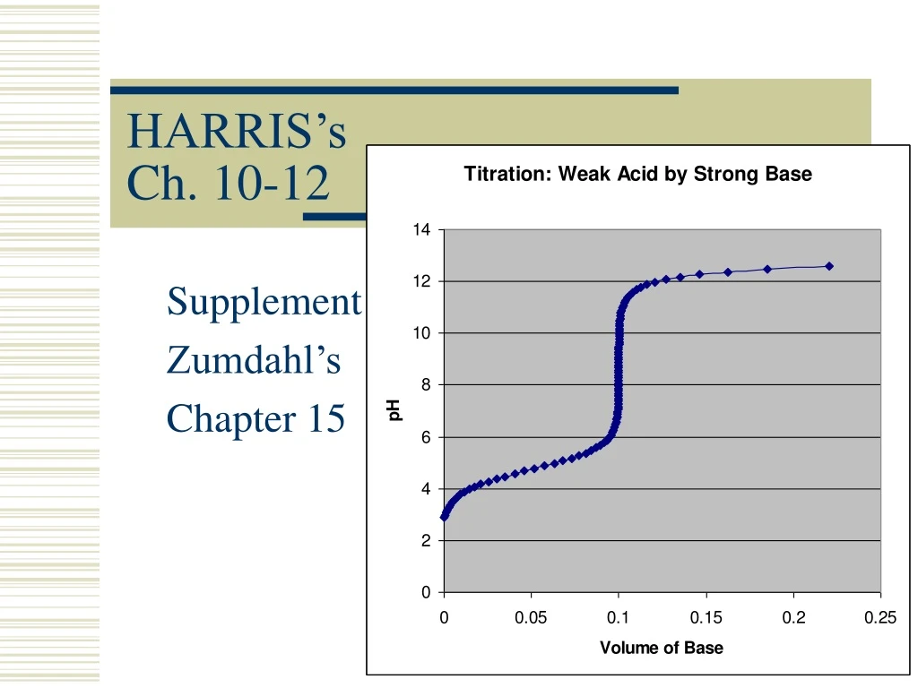
Spreadsheet Titration Curves • Assume Ca and Cb known; plot Vb vs. pH. • Because it’s easier than pH vs. Vb! • [H+] + [Na+] = [A –] + [OH –] • [Na+] = Cb Vb / Vtotal = Cb Vb / ( Va + Vb ) • [A –] = A¯ Fa = A¯ Ca Va / ( Va + Vb ) • Cb Vb / ( Ca Va ) • = {A¯ – ([H+]–[OH–])/Ca} / {1+([H+]–[OH–])/Cb}
Only Somewhat Twisted • = {A¯ – ([H+]–[OH–])/Ca} / {1+([H+]–[OH–])/Cb} • All known if pH is known. • A¯ = Ka / ( [H+] + Ka ) • [OH –] = Kw / [H+] • Therefore Vb = Ca Va / Cb • as a function of pH. • Excel doesn’t care which is the X or Y axis.
“To Diprotica and Beyond” • For weak polyprotic acids and strong bases: • X = 1 – ( [H+] – [OH –] ) / Ca • Xm = {A¯ – ([H+]–[OH–])/Ca} • Xd = {HA¯ + 2A²¯ – ([H+]–[OH–])/Ca} • Xt = {H2A¯ +2HA²¯ +3A³¯ – ([H+]–[OH–])/Ca} • D for triprotic fractional compositions: • D = [H+]³ + K1[H+]² + K1K2[H+] + K1K2K3