Download
1 / 71
860 likes | 1.48k Views
Tree-building methods: Distance vs. Char. Distance-based methods involve a distance metric, such as the number of amino acid changes between the sequences, or a distance score. Examples of distance-based algorithms are UPGMA and neighbor-joining.

E N D
Tree-building methods: Distance vs. Char • Distance-based methods involve a distance metric, such as the number of amino acid changes between the sequences, or a distance score. Examples of distance-based algorithms are UPGMA and neighbor-joining. • Character-based methods include maximum parsimony and maximum likelihood. Parsimony analysis involves the search for the tree with the fewest amino acid (or nucleotide) changes that account for the observed differences between taxa.
Globin • Golbins are first proteins to be sequenced • Hemoglobins • Myoglobin
Myoglobin • Tetrameric hemoglobin • Beta globin subunit • Myoglobin & beta globin
Distance-based tree Calculate the pairwise alignments; if two sequences are related, put them next to each other on the tree
Character-based tree: identify positions that best describe how characters (amino acids) are derived from common ancestors
Tree Construction • Multiple sequences are aligned • Use JC or other models to compute pair-wise evolutionary distances Jukes-Cantor (JC) Kimura 2P Kamura
Tree Construction • From distance matrix, use a clustering method • Join the closest two clusters to form a larger one • Recompute distances between all clusters • Repeat two steps above until all species are connected
Tree from Distance Matix • Given a weighted tree, with weights on edges representing evolutionary distances • Additive distances • di,c+ dc,j= Di,j • Find the nearest leaves – combine to the same parent • Not easy to find neighboring leaves
Reconstructing tree • Shorten all hanging edges of a tree • Reduce length of every hanging edge by the same small amount δ, then distance matrix is reduced by 2δ • Find the leaf with 0 weight and remove the leaf
1 2 3 4 5 Tree-building methods: UPGMA UPGMA is unweighted pair group method using arithmetic mean
1 2 3 4 5 Tree-building methods: UPGMA Step 1: compute the pairwise distances of all the proteins. Get ready to put the numbers 1-5 at the bottom of your new tree.
1 2 3 4 5 Tree-building methods: UPGMA Step 2: Find the two proteins with the smallest pairwise distance. Cluster them. 6 1 2
1 2 3 4 5 Tree-building methods: UPGMA Step 3: Do it again. Find the next two proteins with the smallest pairwise distance. Cluster them. 6 7 1 2 4 5
1 2 3 4 5 Tree-building methods: UPGMA Step 4: Keep going. Cluster. 8 7 6 3 1 2 4 5
1 2 3 4 5 Tree-building methods: UPGMA Step 4: Last cluster! This is your tree. 9 8 7 6 1 2 4 5 3
UMPGMA Method • Distance between two clusters is defined as the mean of the distances between species in the two clusters • Human cluster vs. chimpanzee/pygmy cluster • Mean of human-chimpanzee and human-pygmy distances • Produces a rooted tree • Tree distance between chimpanzee and pygmy is 0.0149/2 • All species end at the right aligned (because the same molecular evolution is assumed in every species) – not used
Distance-based methods: UPGMA trees • UPGMA is a simple approach for making trees. • An UPGMA tree is always rooted. • An assumption of the algorithm is that the molecular • clock is constant for sequences in the tree. If there • are unequal substitution rates, the tree may be wrong. • While UPGMA is simple, it is less accurate than the • neighbor-joining approach. Page 256
Neighbor-Joining (NJ) Method • Additive distance in an unrooted tree • Distance between two species is the sum of branch lengths connecting them • NJ Method • Construct an unrooted tree whose branch lengths are as close to the distance matrix among species • Algorithm • Join two neighbors, and replace them by a new internal node • Keep repeating the step until all species are covered
Making trees using neighbor-joining • The neighbor-joining method of Saitou and Nei (1987) Is especially useful for making a tree having a large number of taxa. • Begin by placing all the taxa in a star-like structure. Page 259
Making trees using neighbor-joining Next, identify neighbors (e.g. 1 and 2) that are most closely related. Connect these neighbors to other OTUs via an internal branch, XY. At each successive stage, minimize the sum of the branch lengths.
Making trees using neighbor-joining Define the distance from X to Y by dXY = 1/2(d1Y + d2Y – d12)
Phylogenetic Trees • Rooted tree provide direction of evolution and its distance • Unrooted tree is less informative • Finding a root • Use known species relationship • If not known, use mid-point method: finding a point on the tree with the mean distance among the tree is identical in either side – assumes the same evolution rate
Tree-building methods: character based Rather than pairwise distances between proteins, evaluate the aligned columns of amino acid residues (characters).
As an example of tree-building using maximum parsimony, consider these four taxa: AAG AAA GGA AGA How might they have evolved from a common ancestor such as AAA?
Tree-building methods: Maximum parsimony 1 AAA AAA AAA AAA AAA AAA AGA AAA AAA 1 1 1 1 2 1 2 1 AAG AAA GGA AGA AAG AGA AAA GGA AAG GGA AAA AGA Cost = 3 Cost = 4 Cost = 4 In maximum parsimony, choose the tree(s) with the lowest cost (shortest branch lengths). Page 261
Parsimony • Use simplest possible explanation of the data, or with fewest assumptions • Binary states: 0 for ancestral, 1 derived character • 0 may be ancestral tetrpod forelimb bone structure • 1 may be the bone structure in the bird wing • C,D posses a derived character, not possessed by A, B • Tree A: the character must have evolved on the + branch • Tree b: evolved once (+), and lost (*) • Tree c: evolved independently (+) on two branches • Parsimony criterion – tree a is the simplest (single state change)
Making trees using character-based methods • The main idea of character-based methods is to find • the tree with the shortest branch lengths possible. • Thus we seek the most parsimonious (“simple”) tree. • Identify informative sites. For example, constant • characters are not parsimony-informative. • Construct trees, counting the number of changes • required to create each tree. For about 12 taxa or • fewer, evaluate all possible trees exhaustively; • for >12 taxa perform a heuristic search. • Select the shortest tree (or trees). Page 260
Small parsimony Problem Small Parsimony Problem Find the most parsimonious labeling of the internal vertices input: Tree T with each leaf labeled by an m-character string output: Labeling of internal vertices of T minimizing the parsimony score • Characters in the string are independent, and the problem can be solved independently for each character • Assume that each leaf is labeled by a single character • Solve for a more general problem • Length of an edge is defined as the Hamming distance • For k-letter alphabet, • dH(v,w) = 0 if v=w; =1, otherwise
Weighted Small Parsimony Problem Weighted Small Parsimony Problem Find the minimal weighted parsimony score labeling of internal vertices input: Tree T with each leaf labeled by a k-letter alphabet, and kxk scoring matrix output: Labeling of internal vertices of T minimizing the weighted parsimony score • David Sankoff Dynamic Programming, 1975 • Internal vertex v with offsprings u and w • si(v) = min{si(u)+δi,t} + min{si(w)+ δj,t}
Parsimony Example • Five species, scored for 6 characters with 0 or 1 state each • Calculate how many changes of state are needed in a tree, for example alpha delta gamma beta epsilon
Reconstruction of Character 1 alpha delta gamma beta epsilon Red: state of 1 Regular: state of 0 alpha delta gamma beta epsilon
Reconstruction of Character 2 alpha delta gamma beta epsilon alpha delta gamma beta epsilon alpha delta gamma beta epsilon
Reconstruction of Character 3 alpha delta gamma beta epsilon alpha delta gamma beta epsilon
Reconstruction of character 4, 5 alpha delta gamma beta epsilon alpha delta gamma beta epsilon
Reconstruction of character 6 alpha delta gamma beta epsilon
Reconstruction with All Changes • Total # of changes, taking random choice for more than one trees • = 1 + 2 + 2 + 2 + 1 + 1 = 9 alpha delta gamma beta epsilon 2,6 5 4 2,5 4 1,3
Most Parsimonious Trees alpha delta gamma beta epsilon 4,5 6 4,5 • Identical, if unrooted 2 alpha 1,3 gamma beta 4,5 4,5 1,3 2 6 delta gamma delta alpha beta epsilon epsilon 6 4,5 4,5 1,3 2
How to determine Branch Lengths • Given an unrooted tree, use the average over all possible reconstructions of each character alpha delta gamma beta epsilon gamma alpha beta 2,6 5 4 1.5 0.5 1 2,5 4 2.5 1 1 1.5 1,3 epsilon delta
Large Parsimony Problem LargeParsimony Problem Find a tree with n leaves having the minimal parsimony score input: An nxm matrix M describing n species, each represented by m-character string output: A tree T with n leaves labeled by n rows of matrix M, and a labeling of the internal vertices with minimal parsimony score over all possible trees and labelings • NP-complete • Greedy heuristics • Start with an arbitrary tree • Move from one tree to another if it lowers parsimony score by nearest neighbor interchange
Modifying Trees • Views
Nearest Neighbor Interchange • Swap two adjacent branches • Erase an interior branch and two branches connected to it
Probabilistic Models • Likelihood ratios • Example: predict helices and loops in a protein • Known info: helices have a high content of hydrophobic residues • ph and pl: frequencies of AA being in the helix or loop • Lh and Ll : likelihoods that a sequence of N AAs are in a helix or a loop • Lh = ∏N ph , Ll = ∏N pl • Rather than likelihoods, their ratios have more info • Lh/Ll : is sequence more or less likely to be a helical or loop region • S = ln(Lh/Ll) = ∑N ln(ph/pl): positive for helical region • Partition a sequence into N-AA segments (N=300)