Download
1 / 32
340 likes | 864 Views
Operations Management Statistical Process Control Supplement 6. Outline. Statistical Process Control (SPC). Mean charts or X -Charts. Range chart or R -Charts. Control charts for attributes. Managerial issues and control charts. Acceptance Sampling. Statistical Process Control (SPC).

E N D
Operations ManagementStatistical Process ControlSupplement 6
Outline • Statistical Process Control (SPC). • Mean chartsor X-Charts. • Range chart or R-Charts. • Control charts for attributes. • Managerial issues and control charts. • Acceptance Sampling.
Statistical Process Control (SPC) • Statistical technique to identify when non-random variation is present in a process. • All processes are subject to variability. • Natural causes: Random variations. • Assignable causes: Correctable problems. • Machine wear, unskilled workers, poor materials. • Uses process control charts.
Start Take Sample Produce Good Inspect Sample Provide Service Take Samples No Is process in control? Create Stop Process Control Chart Yes Find Out Why Statistical Process Control Steps
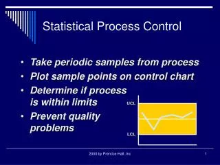
Plot of Sample Data Over Time 80 Upper control limit 60 Sample Value 40 20 Lower control limit 0 1 5 9 13 17 21 Time Process Control Charts
Control Charts • Process is not in control if: • Sample is not between upper and lower control limits. • A non-random pattern is present, even when between upper and lower control limits. • Based on sample being normally distributed.
Distribution of Sample Means Standard deviation of the sample means (mean)
Central Limit Theorem As sample size gets large enough, distribution of meanvalues becomes approximately normal for any population distribution. Central Limit Theorem
Control Chart Types Control Categorical or Discrete Numerical Data Charts Continuous Numerical Data Variables Attributes Charts Charts R P C X Chart Chart Chart Chart
Quality Characteristics Variables Attributes • Characteristics for which you focus on defects. • Categorical or discrete values. • ‘Good’ or ‘Bad’. • # of defects. • Characteristics that you measure, e.g., weight, length. • Continuous values.
X Chart • Shows sample means over time. • Monitors process average. • Example: Weigh samples of coffee. • Collect many samples, each of n bags. • Sample size = n. • Compute mean and range for each sample. • Compute upper and lower control limits (UCL, LCL). • Plot sample means and control limits.
X Chart Control Limits A2 is from Table S6.1 sample range at time i sample mean at time i
Sample Mean Upper Lower Size, n Factor, A Range, D Range, D 2 4 3 2 1.880 3.268 0 3 1.023 2.574 0 4 0.729 2.282 0 5 0.577 2.115 0 6 0.483 2.004 0 7 0.419 1.924 0.076 8 0.373 1.864 0.136 9 0.337 1.816 0.184 10 0.308 1.777 0.223 Factors for Computing Control Chart Limits
X Chart - Example 2 Each sample is 4 measurements. Determine 3 control limits. sample mean range. 1 5.02 .12 4.96, 5.03, 5.01, 5.08 2 4.99 .08 3 4.97 .13 4 5.03 .18 5 4.99 .14
X Chart - Example 2 5.1 Upper control limit=5.095 Sample Mean 5.0 Lower control limit=4.905 4.9 Time
Example 2 – New Samples sample values mean range 6 5.05, 5.00, 4.80, 4.95 4.95 0.25 7 5.00, 5.10, 5.10, 5.00 5.05 0.10 8 4.80, 5.20, 5.10, 5.00 5.025 0.40 5.1 Upper control limit=5.095 Sample Mean 5.0 Lower control limit=4.905 4.9 Time
R Chart • Shows sample ranges over time. • Sample range = largest - smallest value in sample. • Monitors process variability. • Example: Weigh samples of coffee. • Collect many samples, each of n bags. • Sample size = n. • Compute range for each sample & average range. • Compute upper and lower control limits (UCL, LCL). • Plot sample ranges and control limits.
R Chart Control Limits From Table S6.1 sample range at time i
R Chart - Example 2 Each sample is 4 measurements. Determine 3 control limits. sample mean range 1 5.02 .12 2 4.99 .08 3 4.97 .13 4 5.03 .18 5 4.99 .14 4.96, 5.03, 5.01, 5.08
R Chart - Example 2 0.3 Upper control limit=0.297 Sample Range 0.2 0.1 Lower control limit=0 0 Time
Example 2 – New Samples sample values mean range 6 5.05, 5.00, 4.80, 4.95 4.95 0.25 7 5.00, 5.10, 5.10, 5.00 5.05 0.10 8 4.80, 5.20, 5.10, 5.00 5.025 0.40 0.3 Upper control limit=0.297 Sample Range 0.2 0.1 Lower control limit=0 0 Time
Control Chart Steps • Collect 20 to 25 samples of n=4 or n=5 from a stable process & compute the mean and range. • Compute the overall mean and average range. • Calculate upper and lower control limits. • Collect new samples, and plot the means and ranges on their respective control charts.
Control Chart Steps - Continued • Investigate points or patterns that indicate the process is out of control. Assign causes for the variations. • Collect additional samples and revalidate the control limits.
Example 3 sample values mean range 1 4.9, 5.0, 5.1 5.0 0.2 2 5.2, 5.3, 5.4 5.3 0.2 3 5.5, 5.6, 5.7 5.6 0.2 4 5.8, 5.9, 6.0 5.9 0.2
6.0 Upper control limit = 5.6546 Sample Mean 5.5 Lower control limit = 5.2454 5.0 Time 1.0 Upper control limit = 0.5148 Sample Range 0.5 Lower control limit = 0 0.0 Time Example 3 – Control Charts
Example 4 sample values mean range 1 5.0, 5.0, 5.0 5.0 0.0 2 4.5, 5.0, 5.5 5.0 1.0 3 4.0, 5.0, 6.0 5.0 2.0 4 3.0, 5.0, 7.0 5.0 4.0
7.0 Upper control limit = 6.79025 Sample Mean 5.0 Lower control limit = 3.20975 3.0 Time 6.0 Upper control limit = 4.5045 Sample Range 3.0 Lower control limit = 0 0.0 Time Example 4 – Control Charts
p Chart • Attributes control chart. • Shows % of nonconforming items. • Example: Count # defective chairs & divide by total chairs inspected. • Chair is either defective or not defective.
c Chart • Attributes control chart. • Shows number of defects in a unit. • Unit may be chair, steel sheet, car, etc. • Size of unit must be constant. • Example: Count # defects (scratches, chips etc.) in each chair of a sample of 100 chairs.
Acceptance Sampling • Quality testing for incoming materials or finished goods. • Procedure: • Take one or more samples at random from a lot (shipment) of items. • Inspect each of the items in the sample. • Decide whether to reject the whole lot based on the inspection results.
Acceptance Sampling • Inspecting all items is too expensive. • The larger the sample inspected: • The greater the cost for inspection. • The less likely you are to accept a “bad” lot or to reject a “good” lot. • Key questions: • How many should be inspected in each lot? • How confident are you in the accept/reject decision?