Download
1 / 39
540 likes | 970 Views
Multi Angle Laser Light Scattering (MALS). Theory a nd Practice. Joe, Jan 2012. Scattering of visible light by a single molecule. We begin by using a simple example. The light is monochromatic (filters or laser). The light is linearly polarised (we will remove this restriction later).

E N D
Multi Angle Laser Light Scattering (MALS) Theory and Practice Joe, Jan 2012
Scattering of visible light by a single molecule. We begin by using a simple example. The light is monochromatic (filters or laser). The light is linearly polarised (we will remove this restriction later). The light is propagated along the x axis and polarised with the electric vector, E, in the zdirection. The molecule is at x = 0, y = 0 and z = 0. We assume that λ is so long that we can put the molecule at the origin without having to worry about its size
We can write the equation for the electric vector, E, at point x and time t as in Eq 1: Where λ is the wave length and ν is the frequency. At point x = 0 where the molecule resides, the electric field oscillates with time and this is described by Eq 2: Classically, this oscillating field should produce corresponding oscillation of the electrons within the molecule (dipole). These oscillating charges will cause the molecule to act like a miniature antenna, dispersing some of the energy in directions other than the direction of the incident radiation.
The scattered radiation arising from an oscillating dipole moment can be described by a vector that is determined by the polarisability, α, of the molecule (Eq 3). If the molecule is isotropic, the oscillating dipole moment will be in the direction of the electric vector along the z axis and will act as a source of radiation. The amplitude of the electric field produced by an oscillating dipole, at a distance r and at an angle Φ with respect to the direction of polarisation (the z axis) is given by electromagnetic theory (Eq 4).
The term in square brackets represents the amplitude of the scattered wave. In real terms we measure the intensity and not the amplitude of the scattered wave. The intensity depends on the square of the amplitude. We wish to compare the intensity, i, of the scattered radiation to the intensity, I0, of the incident radiation which is proportional to the square of its amplitude, E0 (Eq 5). Eq 5 tells us a great deal about the scattered radiation. It tells us that the scattered radiation falls of with the square of the distance and that it increases rapidly with decreasing wavelength. It also tells us that the scattered intensity depends on the angle Φ and there is no radiation along the direction in which the dipole oscillates. (The strong dependency of scattering on λ accounts for the blue of the sky, since we observe the sunlight scattered by the air and its contaminants, and the blue is scattered more than the red.)
A graph in polar coordinates of the radiation intensity looks like a doughnut-like surface.
Light scattering radiation using an unpolarised light source When unpolarised radiation is used in light scattering experiments this can be regarded as superposition of many independent waves, polarised in random directions in the yz plane. The resulting polar coordinates surface is a summation of the individual surfaces and it looks like somewhat like a dumbbell with the narrowest part in the yz plane.
The equation for the scattering of unpolarised radiation is (Eq 6): Here θ is the angle between the incident beam and the direction of observation. Evidently, the scattering is symmetrical in the forward and backward directions. Eq 6 provide a completely adequate description of the scattering of light from a single molecule. As it stands, this equation is not much use to us because we wish to study solutions containing many macromolecules.
Scattering from a number of small particles: Rayleigh Scattering If a number, N, of identical molecules, each one is much smaller than the wavelength of the incident light, then the intensity of the light scattered by these molecules (in excess of that scattered by the solvent) is just the sum of all the intensities of all the molecules. Hence we can obtain this intensity by multiplying Eq 6 by N (Eq 7): We can easily measure the the scattered (i) and incident (I0) intensities and the wavelength, λ, and the scattering angle, θ, are known. However, in order for Eq 7 to be useful we need to express the polarisability, α, in terms of some more easily measurable quantity.
It turns out that in the visible frequency range the the polarisability is related to the square of the refractive index. Eq 8 describe this relationship. Where n0 is the refractive index of the solvent, C is the weight concentration (g/ml) of the solute and dn/dC is the specific refractive index increment of the solute (easily measured change in the refractive index, n, with change in C). Inserting Eq 8 into Eq 7 and mathematical manipulations gives rise to the following expression (Eq 9): Where A is the Avogadro’s number and M is the molecular weight of the molecule.
Eq 9 tells us that the excess scattering produced by a solution of macromolecules depends on the product CM as well as on the scattering angle θ. If the solute particles are small enough compared to the wavelength then the scattering is symmetrical with respect to the forward and backward scattering. This type of scattering is called Rayleigh Scattering. We can define a quantity, the Rayleigh ratio (Rθ), which correct for the scattering angle (Eq 10): Then, from Eq 9 we get Eq 11: and: Where:
Eq 11 shows that light scattering measurements can be used to determine the molecular weight. However this equations assume that the macromolecules behave like an ideal solution where the solute molecules are entirely independent of each other. This is not the case with real solutions of macromolecules and the scattering will be modified. A precise calculation of the modification of the scattered light due to the non-ideality of the solution is complicated but leads only to a minor modification of Eq 11. The modification of Eq 11 that accounts for the non-ideality of the solution is a power series about C (Eq 12): Where B is a measure of the non-ideality and is called The Second Virial Coefficient.
Because of the non-ideality of solution of macromolecules the scattering must be measured at several concentrations and the quantity KC/Rθ extrapolated to zero concentration.
The measurement of Rθ is usually carried out in a photometer equipped with a laser that provide a well collimated monochromatic beam. The intensity of the light scattered at a given angle θ is compared to the intensity of the incident light. The solutions must be scrupulously clean because small amount of dust particles will contribute significantly to the scattering (Mapp). In addition, calculations of the molecular weight requires a knowledge of dn/dC. Since the difference in refractive index between dilute solution and pure solvent is very small, a differential refractometer which directly measures the small difference n – n0 is commonly used.
SEC-MALS Classical light scattering as described by Rayleigh theory applies only to molecules that have a radius of gyration (s) smaller than λ/20. Several theoretical approaches have been used to deal with the limitations of Rayleigh theory (Gans, Debey, Zimm). If a scattering particle is not small i.e. s > λ/20 then light scattered from different parts of the particle will reach the detector by traveling different path lengths. The difference in path lengths can lead to destructive interference that reduces the intensity of the scattered light. The net effect is that the scattering diagram for large particles is reduced in intensity compared to diagram for small particles.
From the scattering diagram it is clear that the amount of intensity reduction due to destructive interference depends on the scattering angle. However, at θ = zero there is no destructive interference of the scattered light. Therefore, to correct for large particle scattering we need to measure the scattering at θ = zero. Unfortunately this is not possible because the θ angle is the angle at which the incident light illuminates the particle and the transmitted light at this angle swamps the scattered light. Because of that we have to measure the scattering at θ > zero and extrapolate the results to θ = zero. In order to do that we need to introduce a new extrapolation function, P(θ), which is referred to as the ‘structure factor’ or ‘structure function’. P(θ) is the ratio of the actual scattering, iθ, to the scattering that would occur off a much smaller particle ,i0θ (Eq 13). At θ = zeroP(θ) = 1 and P(θ) < 1 for all other θ
From Eq 11 it can be shown that (Eq 14): To use this equation we need some information about P(θ). Fortunately this information can be derived from theoretical analysis of large-particle scattering (Eq 15): Where <s2> is the mean-squared radius of gyration. We can now write an expression that describes the scattering from large particles in non-ideal solutions (Eq 16). This equation is the basis for light scattering measurements.
Since the concentration used in SEC-MALS is small (1 – 5 mg/ml) and the sample is further diluted as it passes through the column, the term 2BC becomes negligible, Eq 16 simplifies to Eq 17: In SEC-MALS the differential refractive index detector measures the concentration of the sample, whereas the MALS detector measures simultaneously the light scattered at several angles. A plot of KC/Rθ versus sin2(θ/2) is used to calculate the molecular weight from the intercept at sin2(θ/2) = zero and the radius of gyration from the slope.
Practice Our SEC-MALS setup: DAWN-HELEOS II OptilabTrEX AKTA-FPLC
DAWN-HELEOS II Our instrument: polarised Laser @ 664 nm (no temp control) COMET RI glass = 1.52 Our DAWN-HELEOS has only 8 detectors
Operating the DAWN-HELEOS: • Buffers and samples should be scrupulously cleaned, buffers by filtering (0.2 µmSteriFilters) into clean glassware, samples by centrifuge/filter. • The laser should be switched on 30 min before taking measurements. • For SEC-MALS run the buffer O/N at 0.5 ml min to equilibrate column and signal. • When the scattering signal is stable the noise level should be 20 – 40 µV. • At the end of a run use the inbuilt COMET system to clean the cell under flow. • At the end of the run and if you do not intend to continue using the instrument, switch the laser off.
OptilabTrEX • The Optilab T-rEX is a deflection-based instrument that uses an array of light sensitive detectors in the measurement of dRI. It has a linear array of 512 photodiodes, rather than the traditional two photodiodes used by other deflection-based instruments. This photodiode array allows for unprecedented sensitivity and range. • The Optilab T-rEX contains a flow cell design that allows the measurement of a fluid's absolute Refractive Index (aRI) in addition to the dRI between two fluids. The aRI of a fluid is vital for characterizing a system and is a necessary input parameter for light scattering measurements that determine the molecular mass of molecules in solution. • Since the dRI of liquids depends critically on temperature, the instrument has a system that precisely regulates the temperature of both the flow cell and the optics. • Our instrument is at ~ 664 nm (matched to our MALS instrument). The light source is LED.
Operating the OptilabTrEX: • Swithch the Purge on the before the run for several minutes at the run flow rate until the aRI signal is stable. Note the aRI and turn the Purge off. • Start the run only after the temp and dRI signals are stable. • For SEC-MALS run the buffer O/N at 0.5 ml min to equilibrate column and signal. • When the scattering signal is stable the noise level should be 20 – 40 µV.