Download
1 / 19
200 likes | 238 Views
Explore the significance of Longest Common Prefix Array (LCP) construction algorithms, comparing existing methods to new ones and their practical applications. Discuss space-time tradeoffs and performance metrics in text processing.

E N D
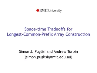
Space-time Tradeoffs forLongest-Common-Prefix Array Construction Simon J. Puglisi and Andrew Turpin (simon.puglisi@rmit.edu.au)
Outline • Refresher on suffix array (SA) and longest-common-prefix array (LCP) basics • Why are they useful? • Existing algorithms for LCP construction • Why do we need new ones? • Two algorithms for LCP construction • Empirical comparison to earlier algorithms • Concise representations of LCP array
The Ubiquitous Suffix Array i suffix 0 toy_boat_toy_boat_toy_boat$ 1 oy_boat_toy_boat_toy_boat$ 2 y_boat_toy_boat_toy_boat$ 3 _boat_toy_boat_toy_boat$ 4 boat_toy_boat_toy_boat$ 5 oat_toy_boat_toy_boat$ 6 at_toy_boat_toy_boat$ 7 t_toy_boat_toy_boat$ 8 _toy_boat_toy_boat$ 9 toy_boat_toy_boat$ 10 oy_boat_toy_boat$ 11 y_boat_toy_boat$ 12 _boat_toy_boat$ 13 boat_toy_boat$ 14 oat_toy_boat$ 15 at_toy_boat$ 16 t_toy_boat$ 17 _toy_boat$ 18 toy_boat$ 19 oy_boat$ 20 y_boat$ 21 _boat$ 22 boat$ 23 oat$ 24 at$ 25 t$ 26 $ SA suffix 26 $ 24 at$ 15 at_toy_boat$ 6 at_toy_boat_toy_boat$ 22 boat$ 13 boat_toy_boat$ 4 boat_toy_boat_toy_boat$ 23 oat$ 14 oat_toy_boat$ 5 oat_toy_boat_toy_boat$ 19 oy_boat$ 10 oy_boat_toy_boat$ 1 oy_boat_toy_boat_toy_boat$ 25 t$ 18 toy_boat$ 9 toy_boat_toy_boat$ 0 toy_boat_toy_boat_toy_boat$ 16 t_toy_boat$ 7 t_toy_boat_toy_boat$ 20 y_boat$ 11 y_boat_toy_boat$ 2 y_boat_toy_boat_toy_boat$ 21 _boat$ 12 _boat_toy_boat$ 3 _boat_toy_boat_toy_boat$ 17 _toy_boat$ 8 _toy_boat_toy_boat$ Suffix Sort
The Longest-Common-Prefix (LCP) Array LCP SA suffix - 26 $ 0 24 at$ 2 15 at_toy_boat$ 10 6 at_toy_boat_toy_boat$ 0 22 boat$ 4 13 boat_toy_boat$ 13 4 boat_toy_boat_toy_boat$ 0 23 oat$ 3 14 oat_toy_boat$ 12 5 oat_toy_boat_toy_boat$ 1 19 oy_boat$ 7 10 oy_boat_toy_boat$ 16 1 oy_boat_toy_boat_toy_boat$ 0 25 t$ 1 18 toy_boat$ 8 9 toy_boat_toy_boat$ 17 0 toy_boat_toy_boat_toy_boat$ 1 16 t_toy_boat$ 10 7 t_toy_boat_toy_boat$ 0 20 y_boat$ 6 11 y_boat_toy_boat$ 15 2 y_boat_toy_boat_toy_boat$ 0 21 _boat$ 5 12 _boat_toy_boat$ 14 3 _boat_toy_boat_toy_boat$ 0 17 _toy_boat$ 9 8 _toy_boat_toy_boat$ LCP[i] = The length of the longest common prefix of suffix SA[i] and SA[i-1]. = |lcp(SA[i-1],SA[i])|, i > 0
Why the Longest-Common-Prefix array? • (SA,LCP,x) == suffix tree • Any bottom-up and top-down traversal (Abouelhoda et al., JDA 2004) • Same asymptotic time bounds, just smaller and faster in practice • Eg., LZ77 factorization (Chen et al., CPM 2007) • Important for disk resident suffix trees • LOFSA (Sinha et al., SIGMOD 2008)
Previous work • Brute force: • for each i \in 1..n-1 work out LCP[i] by comparing t[SA[i-1]..n] to t[SA[i]..n] until we get a mismatch • Expensive if string has regularities, O(n2) in the worst case • Ө(n) time (Kasai et al., CPM 1999) • 13n bytes of space • x[1..n], SA[1..n], ISA[1..n], LCP[1..n] • Ө(n) time (Manzini, SWAT 2004) • Two refinements of Kasai et al.’s algorithm • 9n bytes • 6n + 4Hkn bytes (space usage decreases with text entropy)
The need for new LCP construction algorithms • Prior algorithms use lots of memory • Try to compute LCP[] for the Human Genome • DNA has high entropy, so 9n byte alg is best • 27Gb of RAM • Poor locality of memory reference • Using secondary memory for large inputs implausible • Even in RAM the algorithms are (relatively) slow • Eg., slower than the fastest SA construction algorithms
New Alg: choose a (special) sample of suffixes SA 26 24 15 6 22 13 4 23 14 5 19 10 1 25 18 9 0 16 7 20 11 2 21 12 3 17 8 • Choose a sample of the SA and compute lcp’s • Preprocess L for O(1) time Range Minimum Queries (RMQ) – requires 2n + o(n) bits, after O(n) time preprocessing (Fischer 2008) • Lcp for two non-adjacent suffixes is the minimum value in L[] between them. L S suffix - 15 at_toy_boat$ 0 22 boat$ 4 4 boat_toy_boat_toy_boat$ 0 23 oat$ 1 1 oy_boat_toy_boat_toy_boat$ 0 25 t$ 1 18 toy_boat$ 8 9 toy_boat_toy_boat$ 1 16 t_toy_boat$ 0 11 y_boat_toy_boat$ 15 2 y_boat_toy_boat_toy_boat$ 0 8 _toy_boat_toy_boat$
The sample is defined by a difference cover • A difference cover Dv, modulo v, is a set of integers in the range [0..v) such that for all i \in [0..v), there exist j, k \in Dv such that i = k-j (mod v). • A tool for linear time suffix sorting (Karkkainen et al, JACM, 2006) • |Dv| = O(√v) • δ function defined on Dv: • δ(i,j) = k, i+k and j+k \in Dv (mod v) for any i,j • δ computed in O(1) time and requires O(v) space
New Alg: choose a (special) sample of suffixes SA 26 24 15 6 22 13 4 23 14 5 19 10 1 25 18 9 0 16 7 20 11 2 21 12 3 17 8 • S has O(n/√v) elements (because |Dv| is O(√v)) • In this example, suffixes i such that i mod 7 \in D7 = {1,2,4} have been chosen • Suffixes 1,2,4, 8,9,11, 15,16,18,… L S suffix - 15 at_toy_boat$ 0 22 boat$ 4 4 boat_toy_boat_toy_boat$ 0 23 oat$ 1 1 oy_boat_toy_boat_toy_boat$ 0 25 t$ 1 18 toy_boat$ 8 9 toy_boat_toy_boat$ 1 16 t_toy_boat$ 0 11 y_boat_toy_boat$ 15 2 y_boat_toy_boat_toy_boat$ 0 8 _toy_boat_toy_boat$
S L i+δ(i,j) rank(i+δ(i,j)) l’ = lcp((i+δ(i,j)), (i+δ(i,j))) = RMQL(...) ..... l’ j+δ(i,j) rank(j+δ(i,j)) Using L to compute values in LCP lcp(i,j) i + δ(i,j) j j + δ(i,j) i δ(i,j) δ(i,j) l’ • lcp(i,j) = l’ + δ(i,j)
Computing L • To compute L efficiently we exploit the following simple observation: • If lcp for SA[i] is l, then lcp for SA[i]+v ≥ l-v • The lcp for a given suffix provides a lower bound on the lcp of suffixes which follow it in the string. SA LCP • Overall O(n√v) time and O(n/√v) space to compute L j+v ≥ l-v ..... j l .....
Combining things… • Now computing any LCP[k] requires at most v comparisons and an RMQ on L • To compute LCP over top of SA: • for i = 1 to n do • if lcp(SA[i],SA[i-1]) < v then • LCP[i] = lcp(SA[i],SA[i-1]) • else • LCP[i] = δ(i,j) + RMQL(…) • Total time O(nv); extra space O(n/√v)
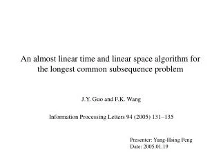
Running Time & Memory Required for 200Mb DNA 200 6n 9n 150 Time (sec) 13n 100 Ours (on disk) Ours (in memory) 50 0 2 4 6 8 10 12 14 Memory (bytes per input character)
Running Time & Memory Required for 200Mb English 200 6n 150 9n Time (sec) Ours (on disk) Ours (in memory) 100 13n 50 0 2 4 6 8 10 12 14 Memory (bytes per input character)
An even better algorithm… • In fact it’s possible to use even less space (and do away with the difference cover as well!) • Requires O(vn) time and O(n/v) space • (Juha Karkkainen, last Friday)
Conclusions • O(nv) time, O(n/√v) space algorithm (using DC) • O(nv) time, O(n/v) space (by rejigging things a bit) • By varying v we have a controlled tradeoff between memory and time • Algorithms are fast and use low memory • Runtime is not greatly effected if the output (and most of the input) resides on disk
Representing LCP in small space • The 2nd algorithm implies a concise representation of the LCP array • nlogn/v bits to store sample suffixes • nlogv bits to store “extra part” • Choosing v = logn → n + nloglogn bits • Sadakane 2001: 6n + o(n) bits
Future Work • Can we eliminate the random access to the text so that algorithm scales unboundedly? • Is there a way to exploit the self-similarity present in the SA (and hence LCP) to further reduce constant factors in the runtime? • What is the concise representation like in practice? Can it be made smaller?