Download
1 / 24
240 likes | 344 Views
Forecasting Global BC and OC Emissions to 2030 and 2050. David G. Streets Argonne National Laboratory, Illinois, USA Workshop on Global Air Pollution Trends to 2030 IIASA, Laxenburg, Austria January 27-28, 2005. Technically, we are most concerned about:

E N D
Forecasting Global BC and OC Emissionsto 2030 and 2050 David G. StreetsArgonne National Laboratory, Illinois, USAWorkshop on Global Air Pollution Trends to 2030IIASA, Laxenburg, AustriaJanuary 27-28, 2005
Technically, we are most concerned about: black carbon (BC), fine aerosol particles generally smaller than 1 micrometer in diameter and mostly elemental carbon, and organic carbon (OC), similar particles in which the carbon is bonded to other atoms. These particles are small enough to travel in the air for a week or more, forming regional air pollution and ultimately being deposited far from the source. The source of carbonaceous aerosols is unburned carbon emitted during inefficient combustion Kathmandu: Brick Kilns
Global distribution of BC emissions in 1996: it’s mostly China, India, and biomass burning (Bond et al., JGR, 2004) China contributes about one-fourth of global BC
Inefficient combustion of coal in small stoves in China produces large quantities of black carbon Coal-burning cook stoves in Xi’an, China
“Give me a future, any future…”(Range of IPCC forecasts of temperature change) A2 and B2 done subsequently 2030 and 2050 done A1B and B1 used in ICAP (Courtesy of Loretta Mickley)
IPCC energy forecasts have been disaggregated to worldregions by the IMAGE team (RIVM, The Netherlands)
EFBC = EFPM x F1.0 x FBC x Fcont EFOC = EFPM x F1.0 x FOC x Fcont where: EFPM = bulk particulate emission factor (usually PM10) F1.0 = fraction of the emissions that are < 1 μm in diameter FBC, FOC = fraction of the particulate matter that is carbon Fcont = fraction of the fine PM that penetrates any control device that might be installed (= 1 if no controls) Calculation of BC and OC emission factors (g kg-1 of fuel burned) for a given tech/fuel combination: (Change with time)
Approach to forecasting BC and OC emissions from the 1996 base-year reference point From Bond et al., JGR, 2004
Level: 1 Change in energy use and fuel type, by sector and world region 2 Improvements in particle control technology 3 Shifts in technology from low-level to higher- level technology/fuel combination 4 Improvements in emission performance of a given technology/fuel combination Major factors influencing future emissions:
Which fuels are used in which sectors in whichparts of the world? (IPCC forecasts used) China photo courtesy of Bob Finkelman Residential coal use has very high BC emissions Level 1 forecasting Residential electricity use from nuclear power has zero BC emissions
Fuel use is partitioned among sectors and technology types(this example is part of the residential sector)
How fast will particle control technology improve (better designs, capture of smaller particles)? Electrostatic precipitator, high collection efficiency Level 2 forecasting Cyclone, low collection efficiency
Particle penetration fractions (Fcont) are included for each type of control device (this example is the power sector) At present, we assume that control technology performance does not vary with world region
A stove is a stove is a…(tech/fuel shifts for a particular energy service) Photo of street vendor’s stove in Xi’an, courtesy of Beverly Anderson Coal-fired, high BC Level 3 forecasting Gas or electric, low BC
Technology splits reflect scenario, regional, and technology differences, and change with time Eight alternative configurations of conventional hard-coal-fired power plants We assume that regional GDP growth determines the rate of replacement of the worst-performing tech/fuel option, with a “nudge” for the environmental scenarios in some cases
Insight, tuk-tuk, or Hummer?(technology performance within a tech/fuel class) Huge variations in fuel efficiency and BC emission rates, often regulatory driven Level 4 forecasting
Emission factors for a given tech/fuel combination are determined using an S-shaped technology penetration curve 1996 current emission factor (Bond/Streets) Shape factor depends on lifetime, build rate, etc. Emission rate (g/kg) “Net” performance in 2030 “Ultimate” performance Time (years)
How to forecast future biomass burning?? The viewis greatly obscured (modified IPCC view used) Many unpredictable factors influence future biomass burning. The IPCC projects only direct anthropogenic influences related to slash-and-burn agriculture, crop residue burning, loss of grassland, etc., driven by regional food demands. We have added natural fires. No accounting for fundamental land-use changes, timber industry practices, climate change influence on fire frequency, and other natural influences.
Components of BC emission changes between 1996 and 2030A1B: technology development overcomes energy growth! (Gg) Energy growth Technology improvement 1996 Bond/Streets Net 2030A1B
Results for all scenarios: a general decline in all cases BC/anthro BC bioburn OC/bioburn OC/anthro
BC emissions in 2050 from anthropogenic activities under the A1B Scenario
BC emissions from open biomass burning in 2050 under the A1B Scenario
A model has been developed to project the global base-year 1996 inventory of Bond/Streets to future years, driven by IPCC regional forecasts of energy, fuel use, and economic activity. The rate of technology development and adoption is an important determinant of future emission levels. The gradual phase-out of inefficient technologies and small-scale solid fuel combustion in the developing world will slowly reduce primary aerosol emissions; more vehicles everywhere will tend to increase emissions Our results suggest that we are headed for a world with stable or lower primary aerosol emissions in the future Conclusions