Download
1 / 61
700 likes | 1.06k Views
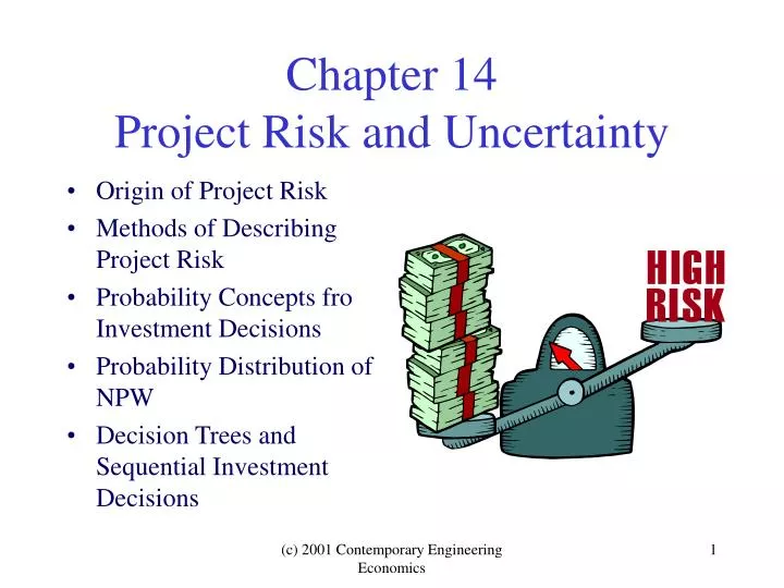
Chapter 14 Project Risk and Uncertainty. Origin of Project Risk Methods of Describing Project Risk Probability Concepts fro Investment Decisions Probability Distribution of NPW Decision Trees and Sequential Investment Decisions. Origins of Project Risk. Risk : the potential for loss

E N D
Chapter 14Project Risk and Uncertainty • Origin of Project Risk • Methods of Describing Project Risk • Probability Concepts fro Investment Decisions • Probability Distribution of NPW • Decision Trees and Sequential Investment Decisions (c) 2001 Contemporary Engineering Economics
Origins of Project Risk • Risk: the potential for loss • Project Risk: variability in a project’s NPW • Risk Analysis: The assignment of probabilities to the various outcomes of an investment project (c) 2001 Contemporary Engineering Economics
Example 14.1 Improving the Odds – All It Takes is $7 Million and a Dream 15 26 3 34 1 39 (c) 2001 Contemporary Engineering Economics
Methods of Describing Project Risk • Sensitivity Analysis: a means of identifying the project variables which, when varied, have the greatest effect on project acceptability. • Break-Even Analysis: a means of identifying the value of a particular project variable that causes the project to exactly break even. • Scenario Analysis: a means of comparing a “base case” to one or more additional scenarios, such as best and worst case, to identify the extreme and most likely project outcomes. (c) 2001 Contemporary Engineering Economics
Example 14.2 - After-tax Cash Flow for BMC’s Transmission-Housings Project – “Base Case” (c) 2001 Contemporary Engineering Economics
(Example 14.2, Continued) (c) 2001 Contemporary Engineering Economics
Example 14.2 - Sensitivity Analysis for Five Key Input Variables Base (c) 2001 Contemporary Engineering Economics
Sensitivity graph – BMC’s transmission-housings project (Example 14.2) $100,000 90,000 Unit Price 80,000 70,000 Demand 60,000 50,000 Salvage value 40,000 Fixed cost Base 30,000 Variable cost 20,000 10,000 0 -10,000 -15% -10% -5% -20% 0% 5% 10% 15% 20% (c) 2001 Contemporary Engineering Economics
Example 14.3 - Sensitivity Analysis for Mutually Exclusive Alternatives (c) 2001 Contemporary Engineering Economics
Ownership cost (capital cost): • Electrical power: CR(10%) = ($29,739 - $3,000)(A/P, 10%, 7) • + (0.10)$3,000 = $5,792 • LPG: CR(10%) = ($21,200 - $2,000)(A/P, 10%, 7) • + (0.10)$2,000 = $4,144 • Gasoline: CR(10%) = ($20,107 - $2,000)(A/P,10%,7) • + (0.10)$2,000 = $3,919 • Diesel fuel: CR(10%) = ($22,263 - $2,200)(A/P, 10%,7) • +(0.1)$2,200 = $4,341 (c) 2001 Contemporary Engineering Economics
b)Annual operating cost as a function of number of shifts per year (M): Electric: $500+(1.56+4.5)M = $500+5.06M LPG: $1,000+(11.22+7)M = $1,000+18.22M Gasoline: $1,000+(13.32+7)M = $1,000+20.32M Diesel fuel: $1,000+(8.14+7)M = $1,000+15.14M (c) 2001 Contemporary Engineering Economics
Total equivalent annual cost: Electrical power: AE(10%) = 6,292+5.06M LPG: AE(10%) = 5,144+18.22M Gasoline: AE(10%) = 4,919+20.32M Diesel fuel: AE(10%) = 5,341+15.14M (c) 2001 Contemporary Engineering Economics
Sensitivity Graph for Multiple Alternatives 12,000 10,000 8000 6000 4000 2000 0 Gasoline Annual Equivalent Cost $ LPG Diesel Electric Power Electric forklift truck is preferred Gasoline forklift truck is preferred 0 20 40 60 80 100 120 140 160 180 200 220 240 260 Number of shifts (M) (c) 2001 Contemporary Engineering Economics
Break-Even Analysiswith unknown Sales Units (X) (c) 2001 Contemporary Engineering Economics
Break-Even Analysis • PW of cash inflows PW(15%)Inflow= (PW of after-tax net revenue) + (PW of net salvage value) + (PW of tax savings from depreciation = 30X(P/A, 15%, 5) + $37,389(P/F, 15%, 5) + $7,145(P/F, 15%,1) + $12,245(P/F, 15%, 2) + $8,745(P/F, 15%, 3) + $6,245(P/F, 15%, 4) + $2,230(P/F, 15%,5) = 30X(P/A, 15%, 5) + $44,490 = 100.5650X + $44,490 (c) 2001 Contemporary Engineering Economics
2. PW of cash outflows: PW(15%)Outflow = (PW of capital expenditure_ + (PW) of after-tax expenses = $125,000 + (9X+$6,000)(P/A, 15%, 5) = 30.1694X + $145,113 3. The NPW: PW (15%) = 100.5650X + $44,490 - (30.1694X + $145,113) =70.3956X - $100,623. 4. Breakeven volume: PW (15%) = 70.3956X - $100,623 = 0 Xb =1,430 units. (c) 2001 Contemporary Engineering Economics
Break-Even Analysis Chart $350,000 300,000 250,000 200,000 150,000 100,000 50,000 0 -50,000 -100,000 Inflow Break-even Volume Profit Outflow PW (15%) Xb = 1430 Loss 0 300 600 900 1200 1500 1800 2100 2400 Annual Sales Units (X) (c) 2001 Contemporary Engineering Economics
Scenario Analysis (c) 2001 Contemporary Engineering Economics
Probability Concepts for Investment Decisions • Random variable: variable that can have more than one possible value • Discrete random variables: Any random variables that take on only isolated values • Continuous random variables: any random variables can have any value in a certain interval • Probability distribution: the assessment of probability for each random event (c) 2001 Contemporary Engineering Economics
Triangular Probability Distribution F(x) 1 f(x) Mo-L (H-L) 2 (H-L) 0 L MoHx 0 LMoHx (a) Probability function (b) Cumulative probability distribution (c) 2001 Contemporary Engineering Economics
Uniform Probability Distribution F(x) 1 f(x) 1 (H-L) 0 LHx 0 LHx (a) Probability function (b) Cumulative probability distribution (c) 2001 Contemporary Engineering Economics
Probability Distributions for Unit Demand (X) and Unit Price (Y) for BMC’s Project (c) 2001 Contemporary Engineering Economics
Cumulative Distribution (for a discrete random variable) (for a continuous random variable) f(x)dx (c) 2001 Contemporary Engineering Economics
Cumulative Probability Distribution for X (c) 2001 Contemporary Engineering Economics
1.0 0.8 0.6 0.4 0.2 0 Probability 1200 1400 1600 1800 2000 2200 2400 2600 Annual Sales Units (X) 1.0 0.8 0.6 0.4 0.2 0 Cumulative Probability Probability that annual sales units will be less than equal to x 1200 1400 1600 1800 2000 2200 2400 2600 Annual Sales Units (X) (c) 2001 Contemporary Engineering Economics
1.0 0.8 0.6 0.4 0.2 0 Probability 40 42 44 46 48 50 52 54 56 Unit Price ($), Y 1.0 0.8 0.6 0.4 0.2 0 Cumulative Probability Probability that annual sales units will be less than equal to y 40 42 44 46 48 50 52 54 56 Unit Price ($), Y (c) 2001 Contemporary Engineering Economics
Measure of Expectation (discrete case) (continuous case) xf(x)dx (c) 2001 Contemporary Engineering Economics
Measure of Variation (c) 2001 Contemporary Engineering Economics
Joint and Conditional Probabilities (c) 2001 Contemporary Engineering Economics
Assessments of Conditional and Joint Probabilities (c) 2001 Contemporary Engineering Economics
Marginal Distribution for X (c) 2001 Contemporary Engineering Economics
After-Tax Cash Flow as a Function of Unknown Unit Demand (X) and Unit Price (Y) (c) 2001 Contemporary Engineering Economics
NPW Function 1. Cash Inflow: PW(15%) = 0.6XY(P/A, 15%, 5) + $44,490 = 2.0113XY + $44,490 2. Cash Outflow: PW(15%) = $125,000 + (9X + $6,000)(P/A, 15%, 5) = 30.1694X + $145,113. 3. Net Cash Flow: PW(15%) = 2.0113X(Y - $15) - $100,623 (c) 2001 Contemporary Engineering Economics
The NPW Probability Distribution with Independent Random Variables (c) 2001 Contemporary Engineering Economics
NPW probability distributions: When X and Y are independent 0.5 0.4 0.3 0.2 0.1 0 Probability 0 20 40 60 80 100 NPW (Thousand Dollars (c) 2001 Contemporary Engineering Economics
Calculation of the Mean of NPW Distribution (c) 2001 Contemporary Engineering Economics
Calculation of the Variance of NPW Distribution (c) 2001 Contemporary Engineering Economics
Comparing Risky Mutually Exclusive Projects (c) 2001 Contemporary Engineering Economics
Comparison Rule • If EA > EB and VA VB, select A. • If EA = EB and VA VB, select A. • If EA < EB and VA VB, select B. • If EA > EB and VA> VB, Not clear. Model 2 vs. Model 3 Model 2 >>> Model 3 Model 2 vs. Model 4 Model 2 >>> Model 4 Model 2 vs. Model 1 Can’t decide (c) 2001 Contemporary Engineering Economics
P{NPW1 > NPW2} (c) 2001 Contemporary Engineering Economics
Decision Tree Analysis • A graphical tool for describing (1) the actions available to the decision-maker, (2) the events that can occur, and (3) the relationship between the actions and events. (c) 2001 Contemporary Engineering Economics
Structure of a Typical Decision Tree A, High (50%) Stock (d ) U(e ,d ,A) o No professional help 1 1 B, Medium (9%) Do not seek advice (e ) C, Low (-30%) Band (d ) o 2 (7.5% return) Seek advice (e ) 1 Decision Node Chance Node Conditional Profit Adding complexity to the decision problem by seeking additional information (c) 2001 Contemporary Engineering Economics
Bill’s Investment Decision Problem • Option 1: 1) Period 0: (-$50,000 - $100) = -$50,100 Period 1: (+$75,000 - $100) - 0.20($24,800) =$69,940 PW(5%)=-$50,100 + $69,940 (P/F, 5%, 1) = $16,510 2) Period 0: (-$50,000 - $100)= -$50,100 Period 1: (+$54,500 - $100)- (0.20)($4,300) = $53,540 PW(5%) = -$50,100 + $53,540 (P/F, 5%, 1) = $890 3) Period 0: (-$50,000 - $100) = -$50,100 Period 1: (+$35,000 - $100) – (0.20)(-$14,800) = $37,940 PW(5%)= - $50,100 + $37,940 (P/F, 5%, 1) = -$13,967 • Option 2: Period 0: (- $50,000 - $150) = -$50,150 Period 1: (+$53,750-$150) = $53,600 PW (5%)= -$50,150 + $53,600 (P/F, 5%, 1) = $898 EMV = $898 Or, prior optimal decision is Option 2 (c) 2001 Contemporary Engineering Economics
Decision tree for Bill’s investment problem A, High (50%) $75,000-$100 B, Medium (9%) $54,500-$100 Stock (d ) 1 C, Low (-30%) • Relevant cash flows before • taxes -$100 $45,000-$100 -$150 -$50,000 (7.5% return) Bond (d ) $53,750-$150 2 (a) 0.25 $16,510 A -$405 B 0.40 $890 d (b) Net present worth for Each decision path 1 $898 C 0.35 $-13,967 $898 d 2 $898 (b) (c) 2001 Contemporary Engineering Economics
Expected Value of Perfect Information (EVPI) • What is EVPI? This is equivalent to asking yourself how much you can improve your decision if you had perfect information. • Mathematical Relationship: EVPI = EPPI – EMV = EOL where EPPI (Expected profit with perfect information) is the expected profit you could obtain if you had perfect information, and EMV (Expected monetary value) is the expected profit you could obtain based on your own judgment. This is equivalent to expected opportunity loss (EOL). (c) 2001 Contemporary Engineering Economics
Expected Value of Perfect Information Prior optimal decision, Option 2 EOL = (0.25)($15,612) + (0.40)(0) + (0.35)(0) = $3,903 EVPI = EPPI – EV = $4,801 - $898 = $3,903 EPPI = (0.25)($16,510) + (0.40)($898) + (0.35)($898) = $4,801 (c) 2001 Contemporary Engineering Economics
Revised Cash flows after Paying Fee to Receive Advice (Fee = $200) 1. Stock Investment Option Period 0: (- $50,000 - $100 - $200)= - $50,300 Period 1: (+$75,000 - $100) – (0.20)($25,000 - $400)= $69,980 PW(5%) = = $50,300 + $69,980(P/F, 5%, 1) = $16,348 2. Bond Investment Option Period 0 (-$50,000 - $150 -$200) = -$50,350 Period 1: (+$53,750 - $150) = $53,600 PW(5%)= -$50,350 + $53,600 (P/F, 5%, 1)= $698 (c) 2001 Contemporary Engineering Economics