Download
1 / 37
370 likes | 628 Views
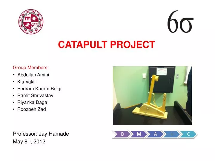
CATAPULT PROJECT Group Members: Abdullah Amini Kia Vakili Pedram Karam Beigi Ramit Shrivastav Riyanka Daga Roozbeh Zad Professor: Jay Hamade May 8 th , 2012. DEFINE PHASE. DEFINE. MEASURE.

E N D
CATAPULT PROJECT Group Members: Abdullah Amini Kia Vakili Pedram Karam Beigi Ramit Shrivastav Riyanka Daga Roozbeh Zad Professor: Jay Hamade May 8th, 2012
DEFINE PHASE DEFINE MEASURE ANALYSE IMPROVE CONTROL Problem statement Problem objective sipoc metrics
PROBLEM STATEMENT • 35% of our Middle East customers that are currently using the latest Catapult-Forza, are returning the product launched in January 2012 for their military training purposes because the distance travelled by the ball doesn’t meet their requested specification range of 200 +- 2 inches. Resulting in a negative profit impact of $10M and reducing market share around 20%.
PROJECT OBJECTIVE • Reducing the product returns from our middle east customers from 35% to 15% by the end of May 2012 to save $5.7M, by modifying and revising the hardware and functionality of the Catapult-Forza , such that it can meet customers shooting specification range (200 +- 2 inches) in every attempt.
S-I-P-O-cprocess 1. Cut The Wood As Per Dimensions 2. Drill Holes In The Wood As Per Dimensions 3. Join The Sides and The Arm To The Base 4. Punch In The Screws and The Bolts 5. Fit The Rubber Bands 6. Fix The Ball Holding Shell
PRIMARY AND SECONDARY METRICS • Primary Metric is used to measure process performance and is the gage used to measure success. • In this case distance travelled by the ball is our primary metric • Secondary Metrics is the vertical distance from the location of our catapult to the floor
Measure phase DEFINE MEASURE ANALYSE IMPROVE CONTROL Gage R&R Normality test Capability test metrics
GAUGE R&R ANALYSIS REQUIREMENTS • 5 Different Parts (Shoot by Catapult) • Black Stone • Marble Ball • White Stone • Paper Clip • Gray Stone • 3 Different Operators (Measuring the Distance) • Randomized Reading
GAGE R&R GRAPHICAL OUTPUT • The following charts are the result of running Gage R&R study for the collected data (measurements) by operators.
GAGE R&R ANALYSIS • Components of Variation “Part-to-Part“ variation is 98.32% . Repeatability and Reproducibility together have a total of 1.67% of variation. This is an ideal result which shows the accuracy and consistency of operators’ measurements. • R-Chart by Operators It shows all the measurements performed by different operators. Most measurements that were recorded were very close to the average. • X-Bar Chart by Operators The above X-Bar chart shows that some points are inside the control limits. This means these parts variations (third and fourth parts) are not easy to detect. This chart shows our measurement system is making it difficult to measure part to part differences for part three and four for operator one and two but for operator three just part three is inside the limit and difficult to measure .
GAGE R&R ANALYSIS • Results by Parts The measurements that were taken should vary little from each other. Most measurements that were recorded were very close to the average. The Marble ball readings were the most accurate measurements recorded compared to other parts. • Results by Operators The above chart shows the measurement of each part by each operator. In this case the total number of measurement is 15 (5 Parts x 3 Times). The variations between the measurements of each operator is different. The averages are varying for all 3 Operators. Ideally, the variation in measurement of each operator must be the Same. Reasons are Human Errors, Reduction in Elasticity Of The Rubber Band, Instrument Related Errors, Setup For Measurements • Operators / Parts Interaction Average measurement taken by each operator on each part The variation in the measurement is very low
NORMALITY TEST • Select one part for the Normality Test – Marble Ball • Shoot the ball 30 times from the catapult
Analyze phase DEFINE MEASURE ANALYSE IMPROVE CONTROL Process Map Fishbone diagram C&E Analysis FMEA
DETAILED PROCESS MAP Arm Holder Base Arms Object Holder Arm Holder Base Arms Partially Assembled Catapult Catapult-Forza Cut the Wood as per Dimension Drill Holes Assembly of Arms and Base Fix the Rubber band & Install Angel Measurement Input Input Input Input • Wood C • Tools C • Blue Prints S • Operator N • Supplier S • Base C • Arms C • Arm Holder C • Object Holder C • Tools C • Blue Prints S • Operator N • Arms C • Base C • Arm Holder C • Position of Pin on Fixed Arm C • Position of Pin on Moving Arm C • Tools C • Blue Prints S • Assembly of Catapult C • Rubber band N • Nuts S • Bolts S • Operator N • Angel of moving Arm C
TOP 3 CAUSES • Angel of Moving Arm • Position of Pin on Fixed Arm • Position of Pin on Moving Arm
Improve phase DEFINE MEASURE ANALYSE IMPROVE CONTROL DOE Interaction Plot Pareto Chart Equation
PARETO CHART OF THE EFFECTS • Minitab displays the absolute value of the Effects on the Pareto Chart • The Chart shows which Effects are active meaning which effects are affecting the distance • The plot shows that Position of the Pin on Stationary Arm is active • Chart also shows the interaction between other factors
INTERACTION PLOT FOR RESULTS • This Graph helps us look at the Significant Interaction between the 3 sources of error • It tells us how big each effect is • Here, In order to get highest yield from our experiment, angle should be set to point 4, position of the stationary pin should be set to 3 and position of the pin on the moving arm to 3
NORMAL PLOT OF THE EFFECTS • The Normal Plot and Pareto Chart shows which effects influence the yield • The graphs shows all the points are outside the fitted line hence active
MAIN EFFECTS PLOT FOR RESULTS • The Plot shows the effects of changing angle and the positions of the pins on the stationary and moving arm • Here we can see that the Positions of the Pins on the Stationary Arm has the major effect on achieving the target spec and then the Position of the Pin on Moving Arm
CUBE PLOT FOR RESULT • From The Cube Plot, In order To Get The Desired Specification Of The Distance i.e. 78.74 inches, • The Angle should be set to point 4 • The Position of the Pin on the Fixed Arm should be between 1 & 3 • The Position of the Pin on the Stationary Arm should also be between 1 & 3
OPTIMIZATION PLOT • As the name suggest, the plot gives the combination of effects for optimum efficiency, i.e. to meet the desired specifications • In our case, • The Angles should be set to point 4 • The Position of the Pin on the Fixed Arm should be at point 1.7822 • The Position of the Pin on the Stationary Arm should be at point 1.4021
FORMULA Y = F(X) Target Value= F (Position of Pin On Stationary Arm) + F (Position of Pin On Moving Arm) + F (Angle Of Moving Arm) 78.74 = F(1.7822) + F(1.4021) + F(4.0)
Control Phase DEFINE MEASURE ANALYSE IMPROVE CONTROL IMR Chart X Bar – R chart Normality Plot Conclusion
BLUE PRINT WITH MODIFICATIONS 1.7822 1.4021 4
PROCESS NORMALITY PLOT The Normality plot shows a scatter plot of the measurements and the line of best fit. More points are on and closer to the line of best fit comparatively. The P-Value is 0.703 which proves our distribution is normal.
PROCESS CAPABILITY PLOT The Process Capability test shows that the Cpk is 0.51 which is better than our previous Cpk value. However the process is still not capable.
Xbar-R CHART • The X bar chart shows • The points are the average of each subgroup • The red control limits which shows the process in under control as none of the points are outside the UCL and LCL • The green line is the overall average which is the mean X bar which is 78.537 • The R bar chart shows • The points as difference in the largest and the smallest measurement within each sub group • The green line is the grand average of each points which is the mean R bar which is 0.753 • The red lines are the upper and lower control limits and here none of the points are outside the UCL and LCL
CURRENT SIGMA LEVEL • Sigma Level = Cpk x 3 • Current Cpk = 0.51 • Current Sigma Level = 0.51 x 3 = 1.53
CONCLUSION • All the Data points in the Xbar and R chart are within the UCL and LCL hence the process is in control. • The Cpk of the process has increased from -7.82 to 0.51. • Further Analysis is required to increase the Cpk and Sigma level.