Download
1 / 19
190 likes | 653 Views
2. . Most slides are explained in detail in the

E N D
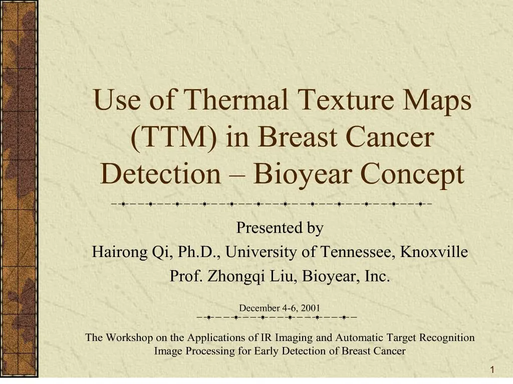
1. 1 Use of Thermal Texture Maps (TTM) in Breast Cancer Detection � Bioyear Concept Presented by
Hairong Qi, Ph.D., University of Tennessee, Knoxville
Prof. Zhongqi Liu, Bioyear, Inc.
December 4-6, 2001
The Workshop on the Applications of IR Imaging and Automatic Target Recognition Image Processing for Early Detection of Breast Cancer
2. 2
3. 3 TTM Slicing - A New Concept IR images the heat emanating from the heat source transported by the radiation and picked up by the IR on the surface. (FDA definition). Quantifying the heat source from the surface temperature is actually an inverse heat transfer problem. However, this problem is very difficult to solve. Instead of going through all the hassles of solving this inverse problem directly, we developed a concept which can quantify the heat source by using the thermal-electric analogue.IR images the heat emanating from the heat source transported by the radiation and picked up by the IR on the surface. (FDA definition). Quantifying the heat source from the surface temperature is actually an inverse heat transfer problem. However, this problem is very difficult to solve. Instead of going through all the hassles of solving this inverse problem directly, we developed a concept which can quantify the heat source by using the thermal-electric analogue.
4. 4 Thermal-Electric Analogue The left two figures show that we can make an analogy between thermodynamics systems and the electrical circuit, where the heat source S can be simulated as a battery U_s, the heat loss inside the heat source can be simulated as the heat loss on a resistor R_s. The temperature of the heat source can then correspond to the voltage of the battery, and the heat current to the circuit current. Similarly, we can map the heat source in the air as U_A, and the heat loss as R_A. The set of Ri and Ci correspond to the unit heat resistance and heat capacity along each radiation line. The circuit only shows the analogy for one radiation line.
H(x) is the transfer function and n is the number of resistors used in the circuit. D is the depth of the heat source and R0 is the unit heat loss over a certain media.
The picture to the right shows that the heat pattern on the surface distributed like Gaussian, if assume M1 is homogeneous.
The left two figures show that we can make an analogy between thermodynamics systems and the electrical circuit, where the heat source S can be simulated as a battery U_s, the heat loss inside the heat source can be simulated as the heat loss on a resistor R_s. The temperature of the heat source can then correspond to the voltage of the battery, and the heat current to the circuit current. Similarly, we can map the heat source in the air as U_A, and the heat loss as R_A. The set of Ri and Ci correspond to the unit heat resistance and heat capacity along each radiation line. The circuit only shows the analogy for one radiation line.
H(x) is the transfer function and n is the number of resistors used in the circuit. D is the depth of the heat source and R0 is the unit heat loss over a certain media.
The picture to the right shows that the heat pattern on the surface distributed like Gaussian, if assume M1 is homogeneous.
5. 5 Half Power Point ? Depth Half power point is an important property of Gaussian curve. The property said that the area above the half power point is equal to the area below the half power point. If we slice the Gaussian curve from top to bottom with a fixed interval, the increment of the horizontal radius will not be dramatic until we cross the half power point, as can be seen from the figure. The relative increment at the first layer is 34 pixels, 40 for the 2nd layer, and 116 for the 3rd layer (green block).
So what does half power point have to do with the depth of the heat source? Well, suppose the temperature of the heat source is U0. In the right triangle shown above, the hypotenuse is equal to U0 and then the sides should be equal to 0.707U0. The vertical side is the depth of the heat source, and the horizontal side is the radius of the cross section of the half power point of the Gaussian. In another word, if we can find the half power point, we can find the depth of the heat source.
Each slice of the Gaussian curve corresponds to a temperature deduction of 0.1 degree. There�s a relationship between the deduction of temperature and the distance. Different materials have different correspondence values, e.g. 0.6 degree/cm for bones and 0.1 degree/cm for muscles. Therefore, by slicing the surface temperature at a certain degree per step, we can find the half power point with the accuracy at the level of centimeter.Half power point is an important property of Gaussian curve. The property said that the area above the half power point is equal to the area below the half power point. If we slice the Gaussian curve from top to bottom with a fixed interval, the increment of the horizontal radius will not be dramatic until we cross the half power point, as can be seen from the figure. The relative increment at the first layer is 34 pixels, 40 for the 2nd layer, and 116 for the 3rd layer (green block).
So what does half power point have to do with the depth of the heat source? Well, suppose the temperature of the heat source is U0. In the right triangle shown above, the hypotenuse is equal to U0 and then the sides should be equal to 0.707U0. The vertical side is the depth of the heat source, and the horizontal side is the radius of the cross section of the half power point of the Gaussian. In another word, if we can find the half power point, we can find the depth of the heat source.
Each slice of the Gaussian curve corresponds to a temperature deduction of 0.1 degree. There�s a relationship between the deduction of temperature and the distance. Different materials have different correspondence values, e.g. 0.6 degree/cm for bones and 0.1 degree/cm for muscles. Therefore, by slicing the surface temperature at a certain degree per step, we can find the half power point with the accuracy at the level of centimeter.
6. 6 Slicing This slides shows a synthetic example of how slicing works. The image is taken from a piece of pork fat. An electric bulb is lit and inserted at the center of the port fat as a heat source such that we can control the location of the heat source.
The color map is also shown in the slide. �White� represents the highest temperature and �black� represents the lowest temperature. First of all, an appropriate temperature needs to be found such that white pixels at the center of the pork fat will show up in the next slice. In this example, this appropriate temperature is 20.50. Each following slicing process decreases the highest temperature in the lookup table by 0.1 degree (e.g. the threshold is lowered by 0.1 degree), such that more white pixels can appear. If we come to a point where the increment of the white pixel is dramatic, the half power point is the slice before it. In the example above, the fourth slice generates much more white pixels than the previous three slices. Note that the increment of the white pixel is measured by the increment of the radius of the white cluster.
The depth of the bulb is 3cm, which is the same as the ground truth.This slides shows a synthetic example of how slicing works. The image is taken from a piece of pork fat. An electric bulb is lit and inserted at the center of the port fat as a heat source such that we can control the location of the heat source.
The color map is also shown in the slide. �White� represents the highest temperature and �black� represents the lowest temperature. First of all, an appropriate temperature needs to be found such that white pixels at the center of the pork fat will show up in the next slice. In this example, this appropriate temperature is 20.50. Each following slicing process decreases the highest temperature in the lookup table by 0.1 degree (e.g. the threshold is lowered by 0.1 degree), such that more white pixels can appear. If we come to a point where the increment of the white pixel is dramatic, the half power point is the slice before it. In the example above, the fourth slice generates much more white pixels than the previous three slices. Note that the increment of the white pixel is measured by the increment of the radius of the white cluster.
The depth of the bulb is 3cm, which is the same as the ground truth.
7. 7 Case Study 1 - Simulation This is an animation of the synthetic example.This is an animation of the synthetic example.
8. 8 Diagnosis Protocol Step 1: Grow pattern of lymph nodes in the armpits
Step 2: Size of the abnormal area
Step 3: Appearance of the abnormal area
Step 4: Vascular pattern
Step 5: Nipples and areola pattern
Step 6: Dynamic diagnosis with outside agents (antibiotic, etc.) Besides measuring the depth of the heat source, slicing can also reveal the growth pattern of the white pixels. Different tissues have different growth patterns. By observing this pattern, different tissues can be distinguished as well. For example, the growth patterns of the lymph and the tumor should be like circular, while the growth pattern of blood vessel is along the direction of the blood vessel.
A diagnosis protocol has been designed for radiologists to use Bioyear�s system for early breast cancer detection. Six steps are involved in this protocol. Take the first step as an example, if the lymph nodes in the armpits reveal one heat source with a depth less than 2cm, one abnormal sign (+) will be recorded; if two heat sources appear with a depth less than 2cm and a bilateral temperature difference greater than 0.2 degree, then two abnormal signs (++) will be recorded; etc.
Besides measuring the depth of the heat source, slicing can also reveal the growth pattern of the white pixels. Different tissues have different growth patterns. By observing this pattern, different tissues can be distinguished as well. For example, the growth patterns of the lymph and the tumor should be like circular, while the growth pattern of blood vessel is along the direction of the blood vessel.
A diagnosis protocol has been designed for radiologists to use Bioyear�s system for early breast cancer detection. Six steps are involved in this protocol. Take the first step as an example, if the lymph nodes in the armpits reveal one heat source with a depth less than 2cm, one abnormal sign (+) will be recorded; if two heat sources appear with a depth less than 2cm and a bilateral temperature difference greater than 0.2 degree, then two abnormal signs (++) will be recorded; etc.
9. 9 Case Study 2 � Normal Case This is a normal patient. It is included here as a reference case.This is a normal patient. It is included here as a reference case.
10. 10 Case Study 3 � Vascular Breast This is also a normal case but the patient has vascular breasts, i.e. there are many blood vessels surrounding the breast. Vascular breast usually makes the diagnosis more difficult since tumor might be hidden underneath the blood vessels. This case is to show how blood vessels grow along the direction of the vessels between different slices.This is also a normal case but the patient has vascular breasts, i.e. there are many blood vessels surrounding the breast. Vascular breast usually makes the diagnosis more difficult since tumor might be hidden underneath the blood vessels. This case is to show how blood vessels grow along the direction of the vessels between different slices.
11. 11 Case Study 4 � Small Breast This patient is diagnosed to have ductal carcinoma in the left breast.
From slicing, we observe the following abnormal signs:
1) Lymph node bilateral temperature difference is 0.8 (++++)
2) The tumor is 2cm from the surface (++)
3) The tumor is surrounded by 5 blood vessels (+++)
4) It takes less than 3 slices to have the white pixels surround the nipple (++)This patient is diagnosed to have ductal carcinoma in the left breast.
From slicing, we observe the following abnormal signs:
1) Lymph node bilateral temperature difference is 0.8 (++++)
2) The tumor is 2cm from the surface (++)
3) The tumor is surrounded by 5 blood vessels (+++)
4) It takes less than 3 slices to have the white pixels surround the nipple (++)
12. 12 Case Study 5 � Medium Breast Lobular carcinoma in the left breast.
1) 2cm tumor surrounded by 4 blood vessels. (+++)
2) White pixels surround the nipper in 3 slices (+++)
3) Nipple bilateral temperature difference is 0.8 degree (+)Lobular carcinoma in the left breast.
1) 2cm tumor surrounded by 4 blood vessels. (+++)
2) White pixels surround the nipper in 3 slices (+++)
3) Nipple bilateral temperature difference is 0.8 degree (+)
13. 13 Case Study 6 � Big Breast Lobular carcinoma.
1) Two heat sources at the lymph nodes with a depth greater than 2cm and bilateral temperature difference less than 0.3 degree (+++)
2) Nipple bilateral temperature difference = 1.3 degree (+++)Lobular carcinoma.
1) Two heat sources at the lymph nodes with a depth greater than 2cm and bilateral temperature difference less than 0.3 degree (+++)
2) Nipple bilateral temperature difference = 1.3 degree (+++)
14. 14 Innovations in Medical IR Imaging Capability to detect the metabolic activity within a patient�s body
Increased sensitivity and specificity
US Patent No.: 6,023,637/Feb. 8, 2000
15. 15 Concept Validation Concept validated in China for several applications, including breast cancer
400,000 patients in 5 years (50,000 patients with breast scan)
63 TSI & TMI systems operational in hospitals
3 systems operational in screening centers
Demonstrated early detection of breast cancer
103 breast cancer cases detected by TMI were proved by biopsy.
Among these 103 cases, 92 cases also went through mammography.
Mammography missed 6 out of these 92 cases. 2 of the missed tumor size is 2mm.
Concept validation in US/Canada in initial stages
Ville Marie Breast Cancer Center in Canada
TMI�s diagnosis agrees with Center�s diagnosis on 198 cases out of 200 testing images.
Elliott Mastology Center at Baton Rouge, LA
NIH (Karposi Sarcoma / Angiogenesis) Note that even though 50,000 patients went through breast scan, only 103 cases can be validated. In another word, only these 103 cases went though biopsy. We don�t have records on the number of cancer cases that IR missed in the past 5 years.
Note that even though 50,000 patients went through breast scan, only 103 cases can be validated. In another word, only these 103 cases went though biopsy. We don�t have records on the number of cancer cases that IR missed in the past 5 years.
16. 16 Ovarian Cancer Detection 77 cases
IR can detect tumors at different locations of different sizes
IR: error rate is around 6%
Ultrasound or CT scan: error rate is 3% ~ 5% Note that even though IR has the same error rate as ultrasound and CT, IR doesn�t need body contact and is invasive.Note that even though IR has the same error rate as ultrasound and CT, IR doesn�t need body contact and is invasive.
17. 17 Concept Implementation � Bioyear Prism 2000 System Camera system
Microbolometer (uncooled)
320 x 240
Internal calibration
Sensitivity 0.05oC
TTM software
Smart image processing
Console
Remote control of gantry and bed
Gantry
Bed
rotate 360o left and right
18. 18 The User-Friendly Interface
19. 19 Some Final Words Acknowledgement
Dr. Nick Diakides, Mary Diakides, Dr. William Sander, Dr. Wesley Snyder, Vince Diehl
On-going and future work
Clinical evaluation
Automatic diagnosis
Comments/Questions/Supports?