Download

1 / 46
470 likes | 828 Views
From Digital Photos to Textured 3D Models on Internet Gang Xu Ritsumeikan University & 3D Media Co., Ltd. On-site Demo 3DM Modeler 3DM Stitcher 3DM Calibrator 3DM Viewer Applications Cultural heritage modeling Car & ship modeling 3D Survey Plant Modeling Game Virtual Reality Web design

E N D
From Digital Photos to Textured 3D Models on Internet Gang Xu Ritsumeikan University & 3D Media Co., Ltd.
Applications • Cultural heritage modeling • Car & ship modeling • 3D Survey • Plant Modeling • Game • Virtual Reality • Web design
Outline of This Tutorial • How can 3D be recovered from 2D? • Mathematical Preparations: Solving Linear Equations and Non-linear Optimization • Camera Model and Projection • Epipolar Geometry Between Images • Linear Algorithm for 2-View SFM • Bundle Adjustment (non-linear optimization)
General Strategy • Step 1: Find a linear or closed-form solution • Step 2: Non-linear optimization • A linear or closed-form solution via many intermediate representations usually includes large errors. But this solution can serve as the initial guess in the non-linear optimization.
Part I Mathematical Preparation
Solving Linear Equations (2) • When n=2 • When n>2, the inverse of A does not exist.
Solving Linear Equations (3) Best compromise Define Minimize A+ : pseudo-inverse matrix of A
Solving Linear Homogeneous Equations • When c=0, we cannot use x Define Minimize Under ||x||=1 Solution: Eigen vector associated with the smallest eigen value of
An Example (1) • Fitting a line to a 2D point set • Plane equation • Minimize
An Example (2) x0 e1 a e2
Non-Linear Optimization (1) • Minimize non-linear function
Non-Linear Optimization (2) • High-dimensional space • No closed-form solution • Multiple local minima • Iterative procedure, starting from an initial guess, assuming that f is differentiable everywhere.
An Example: Bundle Adjustment Bundle Adjustment: minimizing difference between observations and back-projections
3 Common Used Algorithms • Gradient Method (1st-order derivative) • Newton Method (2nd-orde derivative) • Levenberg-Marquartd Method = Gradient+Newton, used in 3DM Modeler, 3DM Stitcher and 3DM Calibrator
Part II Camera and Projection
Pinhole Camera • Pinhole Camera lens center Image
Projection Formula y Y y (X,Y,Z) Focal length Z Principal point focus Mirror image Real image
Projection Matrix Homogeneous Coordinates
u Principal point x (u0,v0) v y Image Coordinate Systems Intrinsic parameters Principal point approximately at the image center A: Intrinsic matrix
3D Coordinate Transform Z’ X’ Y’ Object coordinate system Rotation R Translation t Z X Y Camera coordinate system
From Object Coordinates to Pixel Coordinates Z’ X’ u Y’ v F
What Is Unknown? • Intrinsic Parameters: focal length f • Extrinsic Parameters: Rotation matrix R, translation vector t
Rotation Representations r/||r|| ||r|| • 3×3 Rotation MatrixR • Satisfying • There are only 3 degrees of freedom. • A rotation can be represented by a 3-vector r, with ||r|| representing the rotation amount, and r/||r|| representing the rotation axis. • Others: Euler Angles, Roll-Pitch-Yaw, Quarternion
Part III Epipolar Geometry, Essential Matrix, Fundamental Matrix and Homography Matrix
Epipolar Geometry Between Two Images Epipolar lines Epipolar lines Epipolar plane epipoles F F’
Epipolar Equation F,F’,x,x’ are coplanar. x x’ F F’ t
Essential Matrix E: Essential Matrix
Fundamental Matrix F: Fundamental matrix
Degenerate Cases Lead to Homography • Case 1: t=0 (no translation, only rotation. Panorama- 3DM Stitcher) • Case 2: planar scene (3DM Calibrator) • In both cases: the image can be transformed into another by a homography.
Determining E, F and H Matricesfrom Point Matches • E, F and H can only be determined up to scale. • F (and E) can be linearly determined from 8 or more point matches. • H can be linearly determined from 4 or more point matches.
Part VI A Linear Algorithm for 2-View SFM
Determining Translation from Essential Matrix • Assuming that the intrinsic matrix A is available • First compute Essential matrix • Determining t (up to a scale) from • There are two solutions t and -t
Determining Rotation R • We can consider the problem as determining R from 3 pairs of vectors before and after the rotation
Determining Rotation from n Pairs of Vectors R • Given (pi,pi’), i=1,…,n (n>=2), • Define and minimize • There is a linear solution using SVD. … …
F F’ R,t Determining 3D coordinates • Given R, t, x and x’, determine unknown scales s and s’ such that the two lines “meet” in the 3D space.
F F’ R,t In Front of Both Cameras • s>0, s’>0 in front of both cameras • s>0, s’<0 • s<0, s’>0 • s<0, s’<0
Part V Bundle Adjustment
Coordinate System • All space points and camera positions & camera poses are defined in a common coordinate system.
Match Matrix • Match Matrix w(i,j)=1, if i-th point appears in j-th image; otherwise w(i,j)=0 j 1 2 3 … i 0 1 1 1 1 2 . . 1 1 0
Parameters to Determine • The parameters to determine are • (Xi,Yi,Zi), i=1,…,n. Totally 3n • (tj,rj,fj), j=1,…,m. Totally 7m • Altogether 3n+7m
Initial Guess • LM method needs good initial guesses. • They can be obtained using the previous linear algorithm. • Needs to transform all data into the common coordinate system.
References • Olivier Faugeras: 3D Computer Vision: A Geometry Viewpoint, MIT Press, 1993 • Gang Xu and Zhengyou Zhang: Epipolar Geometry in Stereo, Motion and Object Recognition, Kluwer, 1996 • Richard Hartley and Andrew Zisserman: Multiple View Geometry, Cambridge Univ Press, 2000