Download
1 / 68
700 likes | 994 Views
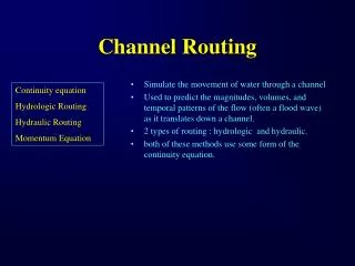
Channel Routing. Simulate the movement of water through a channel Used to predict the magnitudes, volumes, and temporal patterns of the flow (often a flood wave) as it translates down a channel. 2 types of routing : hydrologic and hydraulic.

E N D
Channel Routing • Simulate the movement of water through a channel • Used to predict the magnitudes, volumes, and temporal patterns of the flow (often a flood wave) as it translates down a channel. • 2 types of routing : hydrologic and hydraulic. • both of these methods use some form of the continuity equation. Continuity equation Hydrologic Routing Hydraulic Routing Momentum Equation
Continuity Equation Continuity equation Hydrologic Routing Hydraulic Routing Momentum Equation • The change in storage (dS) equals the difference between inflow (I) and outflow (O) or : • For open channel flow, the continuity equation is also often written as : A = the cross-sectional area, Q = channel flow, and q = lateral inflow
Hydrologic Routing Continuity equation Hydrologic Routing Hydraulic Routing Momentum Equation • Methods combine the continuity equation with some relationship between storage, outflow, and possibly inflow. • These relationships are usually assumed, empirical, or analytical in nature. • An of example of such a relationship might be a stage-discharge relationship.
Use of Manning Equation Continuity equation Hydrologic Routing Hydraulic Routing Momentum Equation • Stage is also related to the outflow via a relationship such as Manning's equation
Hydraulic Routing Continuity equation Hydrologic Routing Hydraulic Routing Momentum Equation • Hydraulic routing methods combine the continuity equation with some more physical relationship describing the actual physics of the movement of the water. • The momentum equation is the common relationship employed. • In hydraulic routing analysis, it is intended that the dynamics of the water or flood wave movement be more accurately described
Momentum Equation Continuity equation Hydrologic Routing Hydraulic Routing Momentum Equation • Expressed by considering the external forces acting on a control section of water as it moves down a channel • Henderson (1966) expressed the momentum equation as :
Combinations of Equations Continuity equation Hydrologic Routing Hydraulic Routing Momentum Equation • Simplified Versions : Unsteady -Nonuniform Steady - Nonuniform Diffusion or noninertial Kinematic Sf = So
Routing Methods • Modified Puls • Kinematic Wave • Muskingum • Muskingum-Cunge • Dynamic Modified Puls Kinematic Wave Muskingum Muskingum-Cunge Dynamic Modeling Notes
Modified Puls • The modified puls routing method is probably most often applied to reservoir routing • The method may also be applied to river routing for certain channel situations. • The modified puls method is also referred to as the storage-indication method. • The heart of the modified puls equation is found by considering the finite difference form of the continuity equation. Modified Puls Kinematic Wave Muskingum Muskingum-Cunge Dynamic Modeling Notes
Modified Puls Modified Puls Kinematic Wave Muskingum Muskingum-Cunge Dynamic Modeling Notes Continuity Equation Rewritten • The solution to the modified puls method is accomplished by developing a graph (or table) of O -vs- [2S/Δt + O]. In order to do this, a stage-discharge-storage relationship must be known, assumed, or derived.
Modified Puls Example • Given the following hydrograph and the 2S/Dt + O curve, find the outflow hydrograph for the reservoir assuming it to be completely full at the beginning of the storm. • The following hydrograph is given:
Modified Puls Example • The following 2S/Dt + O curve is also given:
Modified Puls Example • A table may be created as follows:
Modified Puls Example • Next, using the hydrograph and interpolation, insert the Inflow (discharge) values. • For example at 1 hour, the inflow is 30 cfs.
Modified Puls Example • The next step is to add the inflow to the inflow in the next time step. • For the first blank the inflow at 0 is added to the inflow at 1 hour to obtain a value of 30.
Modified Puls Example • This is then repeated for the rest of the values in the column.
Modified Puls Example • The 2Sn/Dt + On+1 column can then be calculated using the following equation: Note that 2Sn/Dt - On and On+1 are set to zero. 30 + 0 = 2Sn/Dt + On+1
Modified Puls Example • Then using the curve provided outflow can be determined. • In this case, since 2Sn/Dt + On+1 = 30, outflow = 5 based on the graph provided.
Modified Puls Example • To obtain the final column, 2Sn/Dt - On, two times the outflow is subtracted from 2Sn/Dt + On+1. • In this example 30 - 2*5 = 20
Modified Puls Example • The same steps are repeated for the next line. • First 90 + 20 = 110. • From the graph, 110 equals an outflow value of 18. • Finally 110 - 2*18 = 74
Modified Puls Example • This process can then be repeated for the rest of the columns. • Now a list of the outflow values have been calculated and the problem is complete.
MuskingumMethod Modified Puls Kinematic Wave Muskingum Muskingum-Cunge Dynamic Modeling Notes Sp = K O PrismStorage Sw = K(I - O)X WedgeStorage S = K[XI + (1-X)O] Combined
Muskingum,cont... Substitute storage equation, S into the “S” in the continuity equation yields : Modified Puls Kinematic Wave Muskingum Muskingum-Cunge Dynamic Modeling Notes S = K[XI + (1-X)O] O2 = C0 I2 + C1 I1 + C2 O1
Muskingum Notes : • The method assumes a single stage-discharge relationship. • In other words, for any given discharge, Q, there can be only one stage height. • This assumption may not be entirely valid for certain flow situations. • For instance, the friction slope on the rising side of a hydrograph for a given flow, Q, may be quite different than for the recession side of the hydrograph for the same given flow, Q. • This causes an effect known as hysteresis, which can introduce errors into the storage assumptions of this method. Modified Puls Kinematic Wave Muskingum Muskingum-Cunge Dynamic Modeling Notes
Estimating K • K is estimated to be the travel time through the reach. • This may pose somewhat of a difficulty, as the travel time will obviously change with flow. • The question may arise as to whether the travel time should be estimated using the average flow, the peak flow, or some other flow. • The travel time may be estimated using the kinematic travel time or a travel time based on Manning's equation. Modified Puls Kinematic Wave Muskingum Muskingum-Cunge Dynamic Modeling Notes
Estimating X Modified Puls Kinematic Wave Muskingum Muskingum-Cunge Dynamic Modeling Notes • The value of X must be between 0.0 and 0.5. • The parameter X may be thought of as a weighting coefficient for inflow and outflow. • As inflow becomes less important, the value of X decreases. • The lower limit of X is 0.0 and this would be indicative of a situation where inflow, I, has little or no effect on the storage. • A reservoir is an example of this situation and it should be noted that attenuation would be the dominant process compared to translation. • Values of X = 0.2 to 0.3 are the most common for natural streams; however, values of 0.4 to 0.5 may be calibrated for streams with little or no flood plains or storage effects. • A value of X = 0.5 would represent equal weighting between inflow and outflow and would produce translation with little or no attenuation.
Did you know? Lag and K is a special case of Muskingum -> X=0!
More Notes - Muskingum Modified Puls Kinematic Wave Muskingum Muskingum-Cunge Dynamic Modeling Notes • The Handbook of Hydrology (Maidment, 1992) includes additional cautions or limitations in the Muskingum method. • The method may produce negative flows in the initial portion of the hydrograph. • Additionally, it is recommended that the method be limited to moderate to slow rising hydrographs being routed through mild to steep sloping channels. • The method is not applicable to steeply rising hydrographs such as dam breaks. • Finally, this method also neglects variable backwater effects such as downstream dams, constrictions, bridges, and tidal influences.
Muskingum Example Problem • A portion of the inflow hydrograph to a reach of channel is given below. If the travel time is K=1 unit and the weighting factor is X=0.30, then find the outflow from the reach for the period shown below:
Muskingum Example Problem • The first step is to determine the coefficients in this problem. • The calculations for each of the coefficients is given below: C0= - ((1*0.30) - (0.5*1)) / ((1-(1*0.30) + (0.5*1)) = 0.167 C1= ((1*0.30) + (0.5*1)) / ((1-(1*0.30) + (0.5*1)) = 0.667
Muskingum Example Problem C2= (1- (1*0.30) - (0.5*1)) / ((1-(1*0.30) + (0.5*1)) = 0.167 • Therefore the coefficients in this problem are: • C0 = 0.167 • C1 = 0.667 • C2 = 0.167
Muskingum Example Problem • The three columns now can be calculated. • C0I2 = 0.167 * 5 = 0.835 • C1I1 = 0.667 * 3 = 2.00 • C2O1 = 0.167 * 3 = 0.501
Muskingum Example Problem • Next the three columns are added to determine the outflow at time equal 1 hour. • 0.835 + 2.00 + 0.501 = 3.34
Muskingum Example Problem • This can be repeated until the table is complete and the outflow at each time step is known.
Muskingum Example - Tenkiller Look at R-5
Reach at Outlet K = 2 hrs X = 0.25
Let’s Alter XK = 2 hrs. K = 2 hrs X = 0.25 K = 2 hrs X = 0.5
And Again.... K = 2 hrs X = 0.5 K = 2 hrs X = 0.05
Muskingum-Cunge • Muskingum-Cunge formulation is similar to the Muskingum type formulation • The Muskingum-Cunge derivation begins with the continuity equation and includes the diffusion form of the momentum equation. • These equations are combined and linearized, Modified Puls Kinematic Wave Muskingum Muskingum-Cunge Dynamic Modeling Notes
Muskingum-Cunge“working equation” where : Q = discharge t = time x = distance along channel qx = lateral inflow c = wave celerity m = hydraulic diffusivity Modified Puls Kinematic Wave Muskingum Muskingum-Cunge Dynamic Modeling Notes
Muskingum-Cunge, cont... • Method attempts to account for diffusion by taking into account channel and flow characteristics. • Hydraulic diffusivity is found to be : Modified Puls Kinematic Wave Muskingum Muskingum-Cunge Dynamic Modeling Notes • The Wave celerity in the x-direction is :
t X Solution of Muskingum-Cunge • Solution of the Method is accomplished by discretizing the equations on an x-t plane. Modified Puls Kinematic Wave Muskingum Muskingum-Cunge Dynamic Modeling Notes
Calculation of K & X Modified Puls Kinematic Wave Muskingum Muskingum-Cunge Dynamic Modeling Notes Estimation of K & X is more “physically based” and should be able to reflect the “changing” conditions - better.
Muskingum-Cunge - NOTES • Muskingum-Cunge formulation is actually considered an approximate solution of the convective diffusion equation. • As such it may account for wave attenuation, but not for reverse flow and backwater effects and not for fast rising hydrographs. • Properly applied, the method is non-linear in that the flow properties and routing coefficients are re-calculated at each time and distance step • Often, an iterative 4-point scheme is used for the solution. • Care should be taken when choosing the computation interval, as the computation interval may be longer than the time it takes for the wave to travel the reach distance. • Internal computational times are used to account for the possibility of this occurring. Modified Puls Kinematic Wave Muskingum Muskingum-Cunge Dynamic Modeling Notes
Muskingum-Cunge Example • The hydrograph at the upstream end of a river is given in the following table. The reach of interest is 18 km long. Using a subreach length Dx of 6 km, determine the hydrograph at the end of the reach using the Muskingum-Cunge method. Assume c = 2m/s, B = 25.3 m, So = 0.001m and no lateral flow.
Muskingum-Cunge Example • First, K must be determined. • K is equal to : Is “c” a constant? • Dx = 6 km, while c = 2 m/s
Muskingum-Cunge Example • The next step is to determine x. • All the variables are known, with B = 25.3 m, So = 0.001 and Dx =6000 m, and the peak Q taken from the table.
Muskingum-Cunge Example • The coefficients of the Muskingum-Cunge method can now be determined. Using 7200 seconds or 2 hrs for timestep - this may need to be changed