Download
1 / 29
290 likes | 373 Views
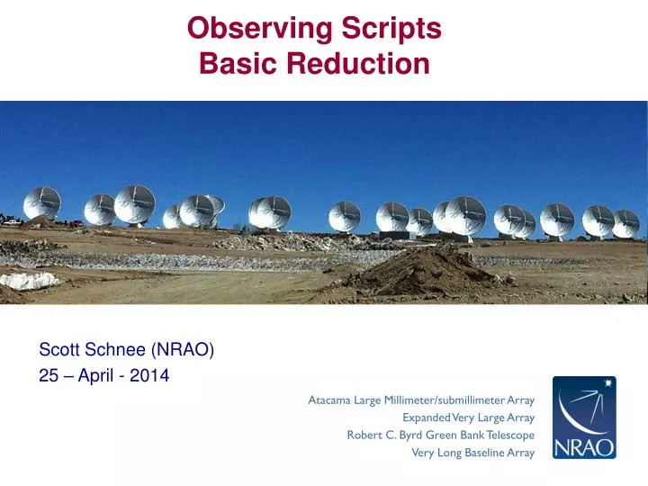
Observing Scripts Basic Reduction. Scott Schnee (NRAO) 25 – April - 2014. b 1. =/ b. phase. The General Idea: Amplitudes and Phases. The visibility is a complex quantity: - amplitude tells “how much” of a certain frequency component - phase tells “where” this component is located.

E N D
Observing ScriptsBasic Reduction • Scott Schnee (NRAO) • 25 – April - 2014
b1 =/b phase The General Idea:Amplitudes and Phases • The visibility is a complex quantity: • -amplitude tells “how much” of a certain frequency component • -phase tells “where” this component is located ALMA Data Workshop – Dec 1st, 2011
The General Idea:Amplitudes and Phases • Each pair of antennas will generate a visibility (amplitude and phase) • Every integration: time interval • Every channel: frequency interval • Goal of calibration is to correct these amplitudes and phases for atmospheric and instrumental effects • Phase corrections are additive • Amplitude corrections are multiplicative • Measurements are baseline-based, but corrections are antenna-based (usually) ALMA Data Workshop – Dec 1st, 2011
The General Idea:Corrupted Data • Variations in the amount of precipitable water vapor (PWV) cause phase fluctuations and result in • Low coherence (loss of sensitivity) • Radio “seeing”, typically 1² at 1 mm • Anomalous pointing offsets • Anomalous delay offsets Patches of air with different water vapor content (and hence index of refraction) affect the incoming wave front differently. ALMA Data Workshop – Dec 1st, 2011
The General Idea:Corrupted Data • The atmosphere can absorb/emit significantly at (sub)millimeter wavelengths, creating phase and amplitude variations that need to be removed from measurement sets • The antennas and other parts of the array also introduce noise into data sets ALMA Data Workshop – Dec 1st, 2011
The General Idea:Calibration • Basic calibration involves observing “calibrators” of known brightness and morphology • Quasars (bright point sources) • Solar system objects (well-characterized, so easily modeled) • Determine corrections that make the observations fit the model • Derive the changes to amplitude and phase (complex gain) vs frequency and time • Apply the corrections from the calibration data to the science target data • Interpolating the derived calibration solutions ALMA Data Workshop – Dec 1st, 2011
What Goes into ALMA Observations? ALMA Data Workshop – Dec 1st, 2011
How to choose calibrators • Bandpass calibrator • Corrects amplitude & phase vs. frequency • Choose brightest quasar in the sky • (Sometimes) assume that corrections are constant in time • Amplitude calibrator • Sets absolute flux of all other sources in observation • Choose something bright, compact, and very well known • Phase calibrator • Corrects amplitude and phase vs. time • Choose quasar that is: • Bright enough to get reasonable signal to noise in (a few) minutes • As close as possible to science target ALMA Data Workshop – Dec 1st, 2011
Other Calibration • Focus observations • Done automatically by ALMA observatory • Data not included in observations delivered to PI • Baseline observations • Done after antennas are moved • Determine the x,y,z position of each antenna in the array • Pointing observations • Done at beginning of observations and after each large (10s of degrees) sky slew • For CARMA, pointing repeated every 2 – 4 hours • WVR observation • Removes short timescale phase fluctuations caused by water vapor in the atmosphere ALMA Data Workshop – Dec 1st, 2011
ALMA WVR Correction Two different baselines Jan 4, 2010 Data WVR Residual • There are 4 “channels” flanking the peak of the 183 GHz water line • Matching data from opposite sides are averaged • Data taken every second, and are written to the ASDM (science data file) • The four channels allow flexibility for avoiding saturation • Next challenges are to perfect models for relating the WVR data to the correction for the data to reduce residual phase noise prior to performing the traditional calibration steps.
First Look at Your Data • In CASA: listobs(vis=‘my_data.ms’) ALMA Data Workshop – Dec 1st, 2011
Task Names • setjy – Set the model for your calibrator • gaincal – Amplitude and phase vs. time solutions • bandpass – Amplitude and phase vs. frequency solutions • fluxscale – Overall amplitude scaling • applycal – Apply solutions from gaincal, bandpass, & fluxscale • plotcal – Plot the amplitude & phase solutions • plotms – Plot the UV data (raw, model, corrected)